10
Frequent Pattern Mining
Frequent pattern mining is an important unsupervised learning task in data mining, with multiple applications. It can be used purely as an unsupervised, exploratory approach to data, and as the basis for finding association rules. It can also be used to find discriminative features for classification or clustering.
In this chapter we describe techniques for building stream pattern mining algorithms. We start (section 10.1) by presenting the main concepts related to pattern mining, the fundamental techniques used in the batch setting, and the concept of a closed pattern, particularly relevant in the stream setting. We then show (section 10.2) in general how to use batch miners to build stream miners and how to use coresets for efficiency. We then concentrate on two instances of the notion of pattern—itemsets and graphs—with algorithms that use the general approach with various optimizations. In section 10.3 we describe several algorithms for frequent itemset mining, and particularly the IncMine algorithm implemented in MOA. In section 10.4 we describe algorithms for frequent subgraph mining, including the AdaGraphMiner implemented in MOA. Section 10.5 provides references for additional reading.
10.1 An Introduction to Pattern Mining
10.1.1 Patterns: Definitions and Examples
In a very broad sense, patterns are entities whose presence or absence, or frequency, indicate ways in which data deviates from randomness. Combinatorial structures such as itemsets, sequences, trees, and graphs, presented next, are widely used to embody this idea. Patterns in this sense can all be viewed as subclasses of graphs [ 255 ]. Our presentation, based on the idea of pattern relation , follows the lines of [ 34 ]; we believe that this allows a more unified presentation of many algorithmic ideas.
Itemsets are subsets of a set of items I = { i 1 , ⋯ ,i n }. In itemsets, the notions of subpattern and superpattern correspond to the notions of subset and superset. The most cited example of itemset mining is the case in which I is the set of products for sale at a supermarket and an itemset is the set of products in one particular purchase. Mining frequent itemsets means finding the sets of products that customers often buy together.
Sequences
in their most basic form are ordered lists of items, such as
⟨
i
3
, i
7
, i
2
, i
10
, i
6
⟩
; both
⟨
i
7
, i
10
⟩
and
⟨
i
3
, i
7
, i
6
⟩
are subsequences of this sequence. An example of usage would be finding sequences of commands frequently issued by the users of some software. A generalization makes every
element of the ordered list an itemset, such as
S
=
⟨
I
1
, I
2
, . . . ,
I
n
⟩
, where each
I
i
is a subset of
I
. The notion of subsequence is correspondingly more difficult:
 is a subsequence of
S
if there exist integers
is a subsequence of
S
if there exist integers
 such that
 .
.
Trees are a special case of acyclic graphs; trees may or may not be rooted, and nodes and edges may or may not be labeled. There are several possible notions of subtree or tree subpattern. An induced subtree of a tree t is any tree rooted at some node v of t whose vertices and edges are subsets of those of t . A top-down subtree of a tree t is an induced subtree of t that contains the root of t . An embedded subtree of a tree t is any tree rooted at some node v of t . See [ 69 , 142 ] for examples and discussions. A practical application of frequent tree mining is related to servers of XML queries, as XML queries are essentially labeled rooted trees. Detecting the frequent subtrees or subqueries may be useful, for example, to classify queries or to optimize, precompute, or cache their answers.
A graph G is a pair formed by a set of nodes V and a set of edges E among nodes. One may add labels to nodes and edges. A common definition of G = ( V, E ) being a subgraph, or graph subpattern, of G ′ = ( V ′ , E ′) is that V ⊆ V ′ and E ⊆ ( V × V ) ∩ E ′. In complex network analysis, motifs are subnetworks that appear recurrently in larger networks, and typically can be used to predict or explain behaviors in the larger network. Finding significant motifs in a network is closely related to mining frequent subgraphs.
Let us now generalize these definitions to a single one. A class of patterns is a set 𝒫 with a relation ≼ that is a partial order: reflexive, antisymmetric, and transitive, possibly with pairs of patterns that are incomparable by ≼ . For patterns p, p ′ ∈ 𝒫 , if p ≼ p ′, we say that p is a subpattern of p ′ and p ′ is a superpattern of p . Also, we write p ≺ p ′ if p is a proper subpattern of p ′, that is, p ≼ p ′ and p ≠ p ′.
The input to our data mining process is a dataset (or stream, in the stream setting) D of transactions, where each transaction s ∈ D consists of a transaction identifier and a pattern. We will often ignore the transaction identifiers and view D as a multiset of patterns, or equivalently a set of pairs ( p, i ) where p occurs i times in D .
We say that a transaction t supports a pattern p if p is a subpattern of the pattern in transaction t . The absolute support of pattern p in dataset D , denoted supp ( p ), is the number of transactions in dataset D that support p . The relative support of p is σ ( p ) = supp ( p )/| D |, where | D | is the cardinality of D . The σ-frequent patterns in a database are those with relative support at least σ in it. Note that the σ -frequent itemsets of size 1 were called σ -heavy hitters in section 4.6.
The frequent pattern mining problem is defined as follows: given a dataset D and a threshold σ in [0, 1], find all σ -frequent patterns in D .
Figure 10.1 presents a dataset of itemsets, and Figure 10.2 shows the frequent, closed, and maximal itemsets of that dataset (closed and maximal patterns will be defined later). For example, patterns de and cde appear in transactions t2, t4, t5 , and no other, and therefore have support 3.
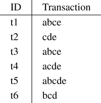
Figure 10.1
Example of an itemset dataset.
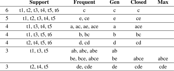
Figure 10.2
Frequent, closed, and maximal itemsets with minimum absolute support 3, or relative support 0.5, for the dataset in
figure 10.1
.
In most cases of interest there is a notion of size , a natural number, associated with each pattern. We assume that size is compatible with the pattern relation, in the sense that if p ≺ p ′ then p is smaller in size than p ′. The size of an itemset is its cardinality, the size of a sequence is the number of items it contains, and the size of a tree or graph is its number of edges. Typically the number of possible patterns of a given size n is exponential in n .
10.1.2 Batch Algorithms for Frequent Pattern Mining
In principle, one way to find all frequent patterns is to perform one pass over the dataset, keep track of every pattern that appears as a subpattern in the dataset together with its support, and at the end report those whose support is larger than the required minimum support. However, the number of subpatterns in the dataset typically grows too fast with dataset size to make this feasible. Therefore, more efficient approaches are required.
A most useful property is antimonotonicity , also known as Apriori property : any subpattern of a frequent pattern is also frequent; equivalently, any superpattern of an infrequent pattern is also infrequent. This suggests the following approach, embodied in the groundbreaking Apriori algorithm for frequent itemset mining [ 9 ]:
- Compute the set F 1 of frequent patterns of size 1, with one pass over the dataset.
- For k > 1, given the set F k −1 ,
2.1. compute the set C k of candidate patterns, those patterns of size k all of whose subpatterns of size k − 1 are in F k −1 ;
2.2. with one pass over the dataset, compute the support of every pattern in C k ; let F k be the subset of patterns in C k that are frequent.
- Stop when F k is empty.
Observe that by the antimonotonicity property we are not losing any truly frequent pattern in step 2.1 when restricting the search to C k . Furthermore, in practice, the number of frequent patterns in F k decreases quickly with k , so step 2.1 becomes progressively faster and the number of passes is moderate. In other words, Apriori [ 9 ] performs a breadth-first exploration of the set of all frequent patterns. It also incorporates other strategies to make the candidate generation phase 2.1 efficient, in particular representing itemsets in lexicographical order.
Other approaches to batch itemset mining differ in the exploration strategy and on the data structures added for efficiency. For example, the FP-growth algorithm [ 131 ] uses a clever data structure called FP-Trees to store the dataset in a compact form using two passes, and then retrieve the frequent itemsets from the FP-tree directly, thus avoiding the expensive candidate generation phase. The Eclat algorithm [ 256 ] can be seen as performing a depth-first search: it associates to each itemset observed a list of the transaction identifiers that support it, then recursively intersects these sets to obtain the lists for larger itemsets.
These and similar ideas have been applied to mining frequent sequences, trees, and graphs. See the surveys cited in section 10.5 for references.
The algorithms sketched above are very clearly batch-oriented: Apriori performs several passes over the dataset; Eclat and FP-growth perform one and two passes, respectively, but it is unclear how they can return results in an anytime way, and they store too many patterns for streaming settings. Before describing approaches that work in streaming, we introduce additional notions that help in reducing memory requirements, in both the batch and stream cases.
10.1.3 Closed and Maximal Patterns
A major problem of frequent pattern mining in practice is that often the algorithm obtains far more patterns than can be later analyzed or used; not only that, the patterns are often redundant or uninteresting in ways that are sometimes obvious and sometimes subtle. See [ 119 ] for proposals of interest measures in pattern mining.
One form of redundancy is to have two frequent patterns p and q such that p ≺ q but p and q have the same or almost the same support. Knowing that p is frequent does not add much when we know that q is frequent. The notions of closed and maximal pattern help reduce redundancy in the output as well as time and memory usage, in both batch and stream miners.
D EFINITION 10.1 A pattern is closed for a dataset D if it has higher support in D than every one of its superpatterns. A pattern is maximal if it is frequent and none of its superpatterns are frequent.
Figure 10.2 shows the frequent closed and frequent maximal itemsets of the dataset in figure 10.1 . For example, ce is closed because it has higher support than its supersets ace , bce , and cde , but e is not, because it has the same support as its superset ce . Pattern ce is frequent but not maximal because its superset cde is also frequent.
Observe that every maximal pattern is closed. It is easy to see (exercise 10.1) that, given all frequent closed patterns, we can retrieve all frequent patterns. If we know moreover the frequency of all closed patterns, we can deduce the frequency of every pattern. There are often far fewer frequent closed patterns than frequent patterns in a dataset. Therefore, algorithms that look for frequent closed patterns without computing all frequent patterns might be much more efficient in time and memory, while providing the same information and less redundant output. This has been verified repeatedly in practice. Maximal patterns only inform us about the border between frequency and infrequency.
CHARM, CLAIM, and FPClose are batch algorithms for mining frequent closed itemsets. BIDE+, ClaSP, and CloSPan are batch miners for frequent closed sequences. CloseGraph finds frequent closed subgraphs. The references can be found in the surveys cited in section 10.5.
10.2 Frequent Pattern Mining in Streams: Approaches
Algorithms for extracting frequent patterns from data streams can be classified according to a number of criteria, including:
- Whether they mine all frequent patterns or only the closed or maximal ones.
- Whether they consider the pattern frequency from the beginning of the stream, or give more importance to recent items, either via sliding windows or some importance decay scheme.
- Whether they update the set of frequent items after each item arrives, or perform batch updates: that is, collect a batch of stream items, then update the data structure that represents frequent patterns using the batch. The choice of batch size is key to performance.
- Whether they are exact or approximate, that is, whether they return exactly the set of patterns that satisfy the frequency condition, or just some approximation of the set. Approximate algorithms may have false positives (infrequent patterns reported as frequent), false negatives (frequent patterns not reported), or both.
We will focus mostly on closed pattern mining using approximate algorithms that perform batch updates. This is because closed pattern mining has a large advantage because of the memory and time reduction it implies. Approximate answers are acceptable in many applications, especially if that saves the high computational cost of exact algorithms. Finally, per-item updates are too slow in most cases and make little difference in the result compared to batch updates.
Algorithms that perform batch updates typically behave as in figure 10.3 . A specific algorithm fixes a summary data structure to remember the current set of patterns being monitored. The summary type will depend on whether the algorithm mines all patterns, or closed ones, or maximal ones. Of course, the summary is also designed from efficiency considerations. The key operations are add ( C, C ′) and remove ( C, C ′). Here, C and C ′ are summary structures representing two pattern datasets D and D ′. The operations should return the summaries corresponding to D ∪ D ′ and D \ D ′, or approximations thereof. Here D \ D ′ denotes multiset difference, the multiset that contains max{0, supp D ( p ) − supp D ′ ( p )} copies of each pattern p . As mentioned already, exact algorithms pay a high computational price for exactness, so add and remove operations that are not exact but do not introduce many false positives or false negatives may be of interest.
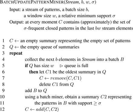
Figure 10.3
A general stream pattern miner with batch updates and sliding window.
The most obvious summary of a dataset D simply forgets the order of transactions in D and keeps the multiset of patterns they contain, or more compactly the set of pairs ( p, supp D ( p )). Then, add and remove are simply multiset union and multiset difference, and are exact. A more sophisticated summary is to keep the pairs ( p, supp D ( p )) for all patterns that are closed in D , even if they do not appear literally in D . This is still exact because the support of all nonclosed patterns can be recovered from the summary. Efficient rules for implementing exact add and remove operations on this representation are given, for example, in [ 34 ].
Example 10.1 Suppose D = { ab, ac, ab }. Its summary in terms of closed patterns is C = {( ab, 2), ( ac , 1), ( a , 3)}, because a is closed in D . If the new batch is D ′ = { ac, bd }, its summary is C ′ = {( ac , 1), ( bd , 1)}, and add ( C, C ′) ideally should return the summary of D ∪ D ′, which is {( ab , 2), ( ac , 2), ( bd , 1), ( a , 4), ( b , 3)}. Observe that add must somehow include ( b , 3), even though b is neither in C nor in C ′.
Since every pattern that occurs literally in a transaction is closed, this summary contains even more distinct patterns than the stream, which seems inefficient. However, if we keep in the summary only the σ -frequent closed patterns, the number of patterns stored decreases drastically, at the cost of losing exactness. In particular, we may introduce false negatives over time, as we may be dropping from a batch summary occurrences of p that are critical to making p σ -frequent in the stream. These false negatives may be reduced by using, in line 15 of the algorithm, some support value σ ′ < σ . Assuming a stationary distribution of the patterns, this makes it less likely that a truly σ -frequent pattern is dropped from a batch because it is not even σ ′-frequent there by statistical fluctuations. Hoeffding’s bound or the normal approximation can be used to bound the rate of false negatives introduced by this approach in terms of σ , σ ′ and batch size (see, for example [ 35 ]).
10.2.1 Coresets of Closed Patterns
Recall from section 9.6 that a coreset of a set C with respect to some problem is a small subset of C such that solving the problem on the coreset provides an approximate solution for the problem on C . We describe an application of the notion of coreset to speed up frequent pattern mining, at the cost of some approximation error. It was proposed for graphs in [ 35 ] as a generalization of closed graphs, but can be applied to other pattern types.
Recall that supp ( p ) and σ ( p ) denote the absolute and relative supports of p . We say that p is δ -closed in D if every superpattern of p has support less than (1 − δ ) supp D ( p ). Closed patterns are the 0-closed patterns and maximal patterns are the 1-closed patterns. This notion is related to others used in the literature, such as the relaxed support in the CLAIM algorithm [ 230 ].
Now define a ( σ, δ ) -coreset of D to be any dataset D ′ ⊆ D such that, for every pattern p ,
- every pattern p occurring in D ′ is σ -frequent and δ -closed in D ,
- and furthermore, if p ∈ D ′ then p occurs as many times in D ′ as in D .
A ( σ, δ )-coreset is a lossy, compressed summary of a dataset. This compression is two-dimensional:
- Minimum support σ excludes infrequent patterns, and
- δ -closure excludes patterns whose support is very similar to that of some subpattern.
Example 10.2 Suppose D = {( ab , 10), ( ac , 5), ( a , 8), ( b , 2)}. A (0, 0.4)-coreset of D is {( ab , 10), ( ac , 5), ( a , 8)}. a is in the coreset because it has support 23 in D , and the supports of both ab and ac are below 0.6 · 23. On the other hand, b is not, because it has support 12 in D and the support of ab is above 0.6 · 12. From the coreset we can only say that the support of b in D is at least 10 and at most 16.
We can build a ( σ, δ )-coreset by greedily choosing a subset of the σ -frequent, δ -closed patterns in D and then putting all their occurrences in D ′. If we do this until it is no longer possible, we obtain a maximal coreset, that is, one that cannot be extended by adding more patterns from D and remain a coreset. See exercise 10.2. For δ = 0, the set of all σ -frequent closed patterns is the unique maximal ( σ , 0)-coreset. If 0 < δ < 1, however, there may be several maximal ( σ, δ )-coresets of D .
A strategy for reducing computation time and memory in the generic algorithm is to keep only summaries of ( σ, δ )-coresets of the batches. Of course, the summaries do not exactly represent the full dataset, not even the σ -frequent patterns in the dataset, so the output will only be approximate.
10.3 Frequent Itemset Mining on Streams
10.3.1 Reduction to Heavy Hitters
In chapter 4 we described a number of sketches for maintaining the heavy hitters of a stream, that is, the elements with relative frequency above a threshold 𝜖 . Such sketches can often be used to maintain the set of frequent patterns in a stream. The extensions need to take into account that it is no longer true that there are at most 1 / 𝜖 frequent elements, because each stream element may generate updates for many patterns.
For example, the paper that presents the Lossy Counting algorithm [ 165 ] also presents an extension to count frequent itemsets. The stream is divided in batches, each batch is mined for frequent itemsets, and the sketch is updated with the result. The error in the frequency estimates of Lossy Counting translates to rates of false positives and negatives in the set of frequent patterns. A similar idea can be developed for the S PACE S AVING sketch (exercise 10.3).
This approach has two disadvantages in some settings: one, it tracks all frequent itemsets rather than frequent closed ones, so it may require large memory. Second, Lossy Counting and Space Saving do not allow removals, so it is not possible to simulate the forgetting effect of a sliding window.
10.3.2 Moment
Moment, by Chi et al. [ 70 ], is a closed frequent itemset miner on a sliding window. It is an exact algorithm: at every moment, it reports exactly the set of frequent closed itemsets in the sliding window.
The method uses a tree structure called a Closed Enumeration Tree to store all the itemsets that are needed at any given moment, where the root is at the top and corresponds to the smallest (empty) itemset. Nodes in the tree belong to one of four types, two on the boundary of frequent and infrequent itemsets, and two on the boundary of closed and nonclosed frequent itemsets:
- Infrequent gateway node: Contains an itemset x that is not frequent, but whose parent node contains an itemset y that is frequent and has a frequent sibling z such that x = y ∪ z .
- Unpromising gateway node: Contains an itemset x that is frequent and such that there is a closed frequent itemset y that is a superset of x , has the same support, and is lexicographically before x .
- Intermediate node: A node that is not an unpromising gateway and contains a frequent itemset that is nonclosed, but has a child node that contains an itemset with the same support.
- Closed node: Contains a closed frequent itemset.
These definitions imply the following properties of Closed Enumeration Trees:
- All supersets of itemsets in infrequent gateway nodes are infrequent.
- All itemsets in unpromising gateway nodes, and all their descendants, are nonclosed.
- All itemsets in intermediate nodes are nonclosed but have some closed descendant.
- When adding a transaction, closed itemsets remain closed.
- When removing a transaction, infrequent items remain infrequent and nonclosed itemsets remain nonclosed.
The core of Moment is a set of rules for adding and removing a transaction from the tree while maintaining these five properties.
10.3.3 FP-S TREAM
FP-S TREAM , by Giannella et al. [ 121 ], is an algorithm for mining frequent itemsets at multiple time granularities from streams. It uses a FP-Tree structure as in FP-growth to store the set of frequent patterns, and a tilted-time window. There are two types of tilted-time window:
- Natural tilted-time window: Maintains the most recent 4 quarters of an hour, the last 24 hours, and the last 31 days. It needs only 59 counters to keep this information.
- Logarithmic tilted-time window: Maintains slots with the last quarter of an hour, the next 2 quarters, 4 quarters, 8 quarters, 16 quarters, and so on. As in Exponential Histograms, the memory required is logarithmic in the length of time being monitored.
FP-S TREAM maintains a global FP-Tree structure and processes transactions in batches. Every time a new batch is collected, it computes a new FP-Tree and adds it to the global FP-Tree.
If only the frequent itemsets in each batch are kept, or only frequent itemsets are maintained in the global FP-Tree structure, many itemsets will be lost, because many nonzero counts that do not reach the minimum required threshold σ will not be included, therefore they are considered effectively zero. It is convenient to keep also some infrequent ones, in case they become frequent in the future. For that purpose, FP-S TREAM uses the notion of subfrequent pattern. A pattern is subfrequent if its support is more than σ ′ but less than σ , for a value σ ′ < σ . FP-S TREAM computes frequent and subfrequent patterns. Pattern occurrences in a batch whose frequency is below σ ′ will not be added to the global FP-Tree, so they will be undercounted and may become false negatives later on. This, however, drops from consideration a large amount of truly infrequent patterns, saving memory and time. A reinforcement of this idea is crucial to the next algorithm we will present.
In summary, FP-S TREAM allows us to answer time-sensitive queries approximately and keeps more detailed information on recent data. It does however consider all frequent itemsets instead of closed ones.
10.3.4 IncMine
The IncMine algorithm for mining frequent closed sets was proposed by Cheng et al. in [ 66 ]. It is approximate and exhibits a controllable, usually small, amount of false negatives, but it is much faster than Moment and FP-S TREAM . Its implementation in MOA, including some details not explicit in [ 66 ], is described in [ 202 ].
At a high level, IncMine maintains a sliding window with batches of the most recent transactions. IncMine aims at reporting the frequent closed itemsets (FCIs) in the window. But it actually stores a superset of those, including some that are not frequent in the current window but may become frequent in the future; we call this set the semi-FCI. Its definition is more restrictive than that of subfrequent patterns in FP-S TREAM .
Stream elements are collected in batches B of some size b . Let w be the number of batches stored in the window, which therefore represents wb transactions.
Let C denote the set of semi-FCIs mined at any given time from the current window. When a new batch of transactions b arrives, C must be updated to reflect the transactions in B and forget the effect of the oldest batch of transactions in the window. Roughly speaking, IncMine performs this by first mining the set C 2 of FCIs in B , and then updating C with the contents of C 2, according to a set of rules that also implements the forgetting of expired transactions. We omit this part of the description, but note that it is crucial for the efficiency of IncMine. Note also that it is specific to itemsets, unlike the following ideas, which are applicable to other types of patterns such as sequences and graphs.
However, a direct implementation of this idea is costly. The number of itemsets that have to be stored in order to perform this task exactly can grow to be very large, because even itemsets that seem very infrequent at this time have to be kept in C , just in case they start appearing more often later and become frequent in the window within the next wb time units or w batches.
IncMine adopts the following heuristic to cut down on memory and computation. Suppose that our minimum support for frequency is σ . If pattern p is frequent in a window of wb batches, by definition it appears at least σwb times in it. Naively, we might expect that it would appear σib times in the first i batches. But it is too much to expect that patterns are so uniformly distributed among batches. However, if p appears far less than σib times in the first i batches, it becomes less likely that the required occurrences appear later in the window, and we might decide to drop pattern p from the window, at the risk that it becomes a false negative some time later. This risk becomes smaller and smaller as i approaches w .
More generally, if σ is the desired minimum support for an FCI, IncMine sets up a schedule of augmented supports r ( i ) for i = 1… b , such that r (1) < r (2) < ⋯ < r ( w − 1) < r ( w ) = 1. When a pattern in the i th batch in the window has frequency below r ( i ) σi b , it is considered unlikely that it will reach frequency σwb after adding w − i batches more, and it is dropped from the current set C .
Therefore, the set C kept by IncMine at a given time is, precisely speaking, the set of σ -frequent closed itemsets in the window plus the set of infrequent closed itemsets that have not been dropped as unpromising in the last w batches. If r ( w ) = 1, this implies that all itemsets that have lived through w batches are σ -frequent in the window, and can be reported as true FCIs. Thus, IncMine may have false negatives, but not false positives, because an itemset reported as frequent is guaranteed to be frequent.
Cheng et al. [ 66 ] propose the linear schedule r ( i ) = ( i − 1) · (1 − r )/( w − 1) + r for some value r < 1. Observe that r (1) = r and r ( w ) = 1. An analysis in [ 202 ] yields another schedule, based on Hoeffding’s bound, that cuts unpromising itemsets much more aggressively while still guaranteeing that at most a desired rate of false negatives is produced, assuming a stationary distribution in the stream.
Let us note also that the implementation in MOA described in [ 202 ] uses CHARM [ 254 ] as the batch miner, partly because of the superior performance reported in [ 254 ] and partly because it can use the well-tested implementation in the Sequential Pattern Mining Framework, SPMF [ 106 ]. The implementation is experimentally shown in [ 202 ] to perform orders of magnitude faster than Moment, with far less memory and with a very small, often negligible, number of false negatives.
10.4 Frequent Subgraph Mining on Streams
Note first that the term graph mining has been used to describe several tasks. A common meaning, which we do not cover here, is the task of mining information such as communities, shortest paths, and centrality measures, from a single large graph such as a social network; the graph arrives an edge at a time, often with edge insertions and deletions. Here we are consistent with the rest of the chapter: each element of the stream is in itself a graph, and the task is to mine the subgraphs of these incoming graphs that are frequent (and, perhaps, closed).
We present two coreset-based algorithms described in [ 35 ], one that implements the general idea for mining patterns over a fixed-size sliding window described in section 10.2, and another one that adapts to change by reporting the approximate set of closed frequent graphs for the recent graphs, those in an adaptive-size sliding window over the stream where the distribution seems to be stationary.
Note that [ 35 ] represents sets of closed graphs in a form equivalent to, but more convenient than, the one implicitly assumed in section 10.2, which was a set of pairs (closed pattern, frequency). The Δ -support of a pattern is its support minus the sum of the absolute supports of all its closed, proper superpatterns; it is called the relative support in [ 35 ], a term we already use with another meaning here.
An interesting property of Δ-support is that, conversely, the absolute support of a closed pattern equals the sum of the Δ-supports of all its closed superpatterns (including itself). This makes adding patterns to a summary much faster. Suppose we have computed the set of closed patterns of a dataset and associated to each its absolute support. To add one occurrence of a pattern p to the summary, we need to increment by 1 the absolute support of p and of all its closed subpatterns. If we instead have kept the Δ-supports of each closed pattern, simply adding 1 to the Δ-support of p implicitly adds 1 to the regular support of all its subpatterns, by the property above. The same argument can be made for removals. Regular supports have to be computed only when the algorithm is asked to output the set of frequent closed graphs, which should happen far more rarely than additions and removals.
If all closed patterns of D are kept in the summary, the Δ-support of p is the number of transactions in D whose pattern is precisely p . However, if the summary is based on a ( σ, δ )-coreset, the missing occurrences of p from the omitted patterns may lead to negative Δ-supports.
10.4.1 W IN G RAPH M INER
The W IN G RAPH M INER algorithm maintains the frequent closed graphs in a sliding window of fixed size, implementing the coreset idea described in section 10.2. Its pseudocode is shown in figure 10.4 . Note that, for brevity, in line 8 we have used set operations in ( G ∪ C ) \ R to denote what really is an application of operation add and an application of operation remove .
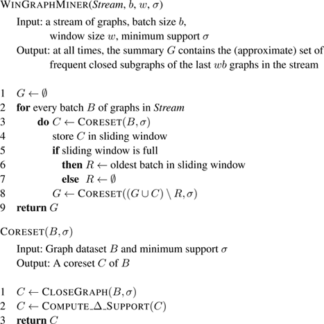
Figure 10.4
The W
IN
G
RAPH
M
INER
algorithm and procedure C
ORESET
.
Every batch of graphs arriving from the stream is mined for closed frequent graphs using some batch miner, and transformed to the relative support representation. Procedure C ORESET implements this idea using the CloseGraph algorithm [ 252 ]. The coreset maintained by the algorithm is updated by adding to it the coreset of the incoming batch. Also, after the first w batches, the window is full, so the algorithm subtracts the coreset of the batch that falls from the sliding window. The subtraction operation can be performed by changing the signs of all the Δ-supports in the subtracted dataset and then adding the coreset summaries.
10.4.2 A DA G RAPH M INER
A DA G RAPH M INER is an extension of the previous method that is able to adapt to changes in the stream, reporting the graphs that are frequent and closed in the current distribution.
There are two versions of this method. One monitors some simple statistic of the global distribution, and shrinks the window when change is detected; in the implementation presented, A DWIN is used as a change detector, and the statistic monitored is the total number of closed graphs. Another version uses a separate A DWIN instance for monitoring the support of each frequent closed subgraph. This version has two advantages: first, it is sensitive to changes in individual graphs that are too small to be noticed in the global distribution. Second, it does not need to keep all the batches in a sliding window in memory, so each graph is stored once, with its A DWIN instance, rather than w times. Although an A DWIN is stored for every graph, this experimentally requires less memory for moderate values of w .
Figure 10.5 shows the pseudocode of A DA G RAPH M INER , where the parameter mode chooses among both versions.
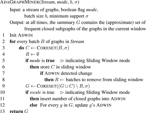
Figure 10.5
The A
DA
G
RAPH
M
INER
algorithm.
10.5 Additional Material
The literature on frequent pattern mining, both batch and in streams, is vast. We prioritize surveys if available, from which many other references can be found. The survey [ 5 ] is most comprehensive on pattern mining; see in particular [ 156 ], chapter 4, on pattern mining in data streams.
Regarding itemsets, [ 67 ] focuses on mining frequent itemsets on streams, and [ 202 ] includes a comparison of the pros and cons of several itemset mining algorithms on streams, besides describing the MOA implementation of IncMine.
For sequence patterns, [ 180 ] is a recent survey, mostly for the batch context. [ 174 , 204 ] are two approaches to sequence mining on data streams.
For frequent subtree mining, [ 24 , 69 , 142 ] present in detail the various notions of “subtree” and survey associated batch algorithms. [ 158 ] presents FQT-Stream, an online algorithm for mining all frequent tree patterns on an XML data stream. [ 34 ] describes the generic approach to stream pattern mining that we have used in this chapter, and applies it in particular to subtree mining.
For subgraph mining, two surveys dealing with the batch case are [ 142 , 206 ]. Two algorithms for mining frequent subgraphs from graphs of streams are gspan [ 251 ] and its extension for closed graphs, CloseGraph [ 252 ]. [ 35 ] proposes the notion of coreset for subgraph mining in graph streams and the algorithms in section 10.2.1. [ 207 ] investigates finding frequent subgraphs in a single large dynamic (streaming) graph.
We have omitted the discussion on association rules , as typically they are obtained by first mining frequent itemsets from the dataset (or stream), then determining the frequent rules from the mined itemset; that is, there is nothing essentially specific to the streaming setting beyond mining frequent itemsets. Association rules, or probabilistic implications, for trees are discussed in [ 23 ], and shown to behave differently from those on sets in several nontrivial ways.
The Sequential Pattern Mining Framework (SPMF) [ 106 ] contains many implementations of pattern mining algorithms, mostly for the batch setting, and mostly in Java. Implementations of IncMine, AdaGraphMiner, and Moment are available from the Extensions section in the MOA website.
10.6 Exercises
Exercise 10.1 Show that: 1. The set of all frequent patterns in a dataset can be derived from its set of closed frequent patterns. 2. If, additionally, we know the support of each frequent closed pattern, we can compute the support of every frequent pattern.
Exercise 10.2 1. Formalize the greedy algorithm sketched in section 10.2.1 to compute a maximal ( σ, δ )-coreset.
2. Consider the dataset D = {( a , 100), ( ab , 80), ( abc , 60), ( abcd , 50)} of itemsets. Find two different maximal (0.1, 0.3)-coresets of D .
Exercise 10.3 If you have studied the S PACE S AVING sketch in chapter 4, think how to adapt it for maintaining the σ -frequent itemsets, counting frequency from the start of the stream. How much memory would it require? Does it have false positives or false negatives, and if so, what bounds can you prove for the error rates?
Exercise 10.4 Without looking at the original paper, give pseudocode for the IncMine algorithm based on the ideas given in this chapter.
Exercise 10.5 Prove that the absolute support of a closed pattern equals the sum of the Δ-supports of all its closed superpatterns (including itself). Hint: Use induction from the maximal patterns down.