9
Clustering
Clustering is an unsupervised learning task that works on data without labels. It consists of distributing a set of instances into groups according to their commonalities or affinities. The main difference versus classification is that the groups are unknown before starting the learning process, and in fact the task is to create them. Uses of clustering include customer segmentation in marketing and finding communities in social networks, among many others.
Many, but not all, clustering methods are based on the assumption that instances are points in some space on which we can impose a distance function d , and that more similar instances are closer in the distance. In many of these methods, a clustering is determined by a set of centroid points in this space. A more formal definition of centroid-based clustering is the following: given a set of instances P belonging to some space X , a distance function d among elements in X , and optionally a number of clusters k , a clustering algorithm computes a set C of centroids or cluster centers C ⊆ P , with | C | = k , that (approximately) minimizes the objective function

where

that is, the distance from x to the nearest point in C .
As indicated, some algorithms require the user to specify a value for k , while others determine a number of clusters by themselves. Observe that by taking k = | P | and assigning an instance to a cluster by itself leads to a clustering with 0 cost, so if k is not bound, some form of penalization on the number of clusters will be required to get meaningful results.
We start by discussing the evaluation problem in clustering and review the popular k -means method. We then discuss three incremental methods that are inspired more or less distantly by k -means: Birch, BICO, and C LU S TREAM . After that, we look at two density-based methods, starting with DBSCAN for nonstreaming data, which leads to Den-Stream for the streaming setting. Finally, we describe two more recent and state-of-the-art tree-based streaming methods, ClusTree and StreamKM++. We provide references and brief discussions of other methods in the closing section 9.7.
9.1 Evaluation Measures
Evaluating a clustering is unfortunately not as unambiguous as evaluating a classifier. There are many different measures of clustering quality described in the literature, maybe too many, which formalize different expectations of what a “good clustering” should achieve.
Measures can be categorized into two distinct groups: structural or internal measures, and ground-truth-based ones, called external measures. The first kind are strictly based on the data points and the clustering obtained. An extensive study of thirty internal measures can be found in [ 178 ], and other studies of external measures include [ 57 , 231 , 250 ]. Some examples are:
- Cohesion: The average distance from a point in the dataset to its assigned cluster centroid. The smaller the better.
- SSQ: The sum of squared distances from data points to their assigned centroids. Closely related to cohesion. The smaller the better.
- Separation: Average distance from a point to the points assigned to other clusters. The larger the better.
- Silhouette coefficient: Roughly speaking, the ratio between cohesion and the average distances from the points to their second-closest centroid. It rewards clusterings where points are very close to their assigned centroids and far from any other centroids, that is clusterings with good cohesion and good separation.
External measures, on the other hand, require knowledge of the “true” clustering of the data points, or ground truth, which by definition is almost always unknown in real scenarios. However, when evaluating new clusterers, one often creates synthetic datasets from a known generator, so it is possible to compare the clustering obtained by the algorithm with the true model. Some measures in these cases are similar to others applied in classification or information retrieval:
- Accuracy: Fraction of the points assigned to their “correct” cluster.
- Recall: Fraction of the points of a cluster that are in fact assigned to it.
- Precision: Fraction of the points assigned to a cluster that truly belong to it.
- Purity: In a maximally pure clustering, all points in the cluster belong to the same ground-truth class or cluster. Formally, purity is
 (number of points in cluster
c
in the majority class for
c
):
(number of points in cluster
c
in the majority class for
c
):
- Cluster Mapping Measure (CMM): A measure introduced by Kremer et al. [ 151 ], specifically designed for evolving data streams, which takes into account the fact that mergers and splits of clusters over time may create apparent errors.
The measures listed above can be easily maintained incrementally storing a constant number of values, if the centroids remain fixed. When the centroids evolve over time, we can resort to turning these values into EWMA accumulators or to evaluating on a sliding window.
9.2 The k -means Algorithm
The k -means (also called Lloyd’s) algorithm is one of the most used methods in clustering, due to its simplicity. Figure 9.1 shows its pseudocode.
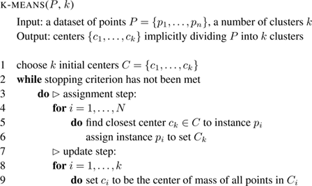
Figure 9.1
The
k
-means clustering algorithm, or Lloyd’s algorithm.
The k -means assumes that the set of points P is a subset of ℜ d for some dimension d , so that points can be added and averaged. The algorithm starts selecting k centroids in an unspecified way—for example, at random. After that, two steps are iterated: first, each instance is assigned to the nearest centroid; second, centroids are recomputed as the mean or center of mass of the examples assigned to it. The process typically stops when no point changes centroid, or after a maximum number of iterations has been performed. The k centroids produced determine the k clusters found by the algorithm.
The greedy heuristic implicit in k -means only guarantees convergence to a local minimum, and the quality of the solution found and the speed of convergence of k -means notoriously depend on the initial random assignment step. k -means++ [ 19 ] improves the stability of the method over the purely random one, using a new initialization step:
1 choose center c 1 to be p 1
2 for i = 2,… ,k
3 do select c i = p ∈ P with probability d ( p,C ) /cost ( C,P ).
In words, the initial center is selected at random, but all subsequent centers are selected with probability proportional to their distance to already selected centers. Spreading out the k initial cluster centers helps in that it leads to faster convergence to better local minima. The stream clustering method StreamKM++ also employs this strategy.
Converting k -means to the streaming setting is not straightforward, since it iterates repeatedly over the dataset. We will see that most stream clustering methods have two phases, one online and one offine. The online phase updates statistics of the data, producing some form of summary or sketch, usually represented as a reduced number of points called microclusters. The offine phase then uses these summaries to compute a final clustering efficiently, either at regular time intervals, or on demand.
9.3 BIRCH, BICO, and C LU S TREAM
These three algorithms are incremental and share a common idea for summarizing the stream in microclusters, in order to cluster them in the offine phase.
Balanced Iterative Reducing and Clustering using Hierarchies (BIRCH) is due to Zhang et al. [ 258 ]. It is the first method for incremental clustering that proposes to use so-called clustering feature (CF) vectors to represent microclusters. Assuming dataset points are vectors of d real numbers, a CF is a triple ( N, LS, SS ) composed of the following items:
- N : number of data points in the CF
- LS : d -dimensional sum of the N data points
- SS : d -dimensional sum of squares of the N data points.
CFs have the following useful properties:
- They are additive: CF 1 + CF 2 = ( N 1 + N 2 , LS 1 + LS 2 , SS 1 + SS 2 ).
- The distance from a point to a cluster, the average intercluster distance, and the average intracluster distance are easy to compute from the CF.
Another feature of BIRCH is its use of CF trees , a height-balanced tree similar to the classical B + tree data structure. It is defined with two parameters: the branching factor B , or maximum number of children that any given node may have, and the leaf radius threshold R . The algorithm maintains the property that all points represented by a leaf fall in a ball of radius R of the centroid there. Every leaf and also every inner node contains a CF vector.
The BIRCH algorithm comprises up to four phases:
Phase 1: Scan all data and build an initial in-memory CF tree
Phase 2: Condense the CF tree into a smaller one (optional)
Phase 3: Cluster globally
Phase 4: Refine clusters (optional and offine, as it requires more passes).
Phases 2, 3, and 4 are the offine part. Phase 3, in particular, performs batch clustering based on the information collected in the CF tree. Phase 1 is the online process, and the one that actually works on the stream. For every arriving point, the algorithm descends the tree, updating the statistics at the CFs of the inner nodes traversed, to reach a leaf closest to the point. Then it checks whether the leaf can absorb it within radius R . If so, the point is “assigned” to the leaf by updating the leaf statistics. If not, a new leaf is created for the new point. This new leaf may cause the parent node to have more than B children; if so, it has to be split into two, and so recursively up to the root. A further rule, not described here, is applied to merge leaves and nodes that may have become too close in the process.
BICO (an acronym for “BIRCH meets coresets for k -means clustering”) is due to Fichtenberger et al. [ 101 ]. It combines the data structure of BIRCH with the theoretical concept of coresets for clustering. Coresets are explained in detail in section 9.6. BIRCH decides heuristically how to group the points into subclusters. The goal of BICO is to find a reduced set that is not only small, but also offers guarantees of approximating the original point set.
C LU S TREAM , by Aggarwal et al. [ 6 ], is designed as an adaptive extension of BIRCH that can deal with changing streams. In C LU S TREAM , nodes of the CF tree maintain CF vectors of the form ( N,LS,SS,LT,ST ), which extend BIRCH CFs with two additional temporal features:
- LT : sum of the timestamps
- ST : sum of squares of the timestamps
The offine phase of C LU S TREAM simply applies k -means periodically to the microclusters at the leaves of the CF tree. The online phase is similar to that of BIRCH, but it takes the recency of clusters into account. It keeps a maximum number of microclusters in memory. If a point requires creating a new microcluster (leaf) and there is no more space available, the algorithm either deletes the oldest microcluster or else merges two of the oldest microclusters. The notion of the “oldest” microcluster is defined taking into account whether there has been significant recent activity in the microcluster. More precisely, statistics LT and ST are used to compute average and standard deviation of its timestamps; assuming a normal distribution of the timestamps, the algorithm can use them to decide whether a desired fraction of the points in the microcluster are older than a desired recency threshold.
The fact that the oldest clusters, not the smallest ones, are chosen for deletion gives C LU S TREAM an interesting property: by looking at microclusters of similar timestamp distributions, we can obtain a snapshot of the clustering in a desired time frame, with more resolution for more recent time frames and less resolution as we move further back in time. This is sometimes called a pyramidal time frame.
9.4 Density-Based Methods: DBSCAN and Den-Stream
Density-based clusterers are based on the idea that clusters are formed not only by overall proximity in distance, but also by the density of connections. They may thus produce clusters that are not spherical, but rather have shapes that adapt to the specific data being clustered.
The DBSCAN algorithm [ 96 ], due to Ester et al., is the best-known density-based, offine algorithm. It is based on the idea that clusters should be built around points with a significant number of points in their neighborhoods. The following definitions formalize this idea:
- The 𝜖 -neighborhood of p is the set of points at a distance 𝜖 or less from p .
- A core point is one whose 𝜖 -neighborhood has an overall weight (fraction of dataset points) of at least μ .
- A density area is the union of the 𝜖 -neighborhoods of core points.
- A point q is directly reachable from p if q is in the 𝜖 -neighborhood of p . Point q is reachable from p if there is a sequence p 1 ,… ,p n such that p 1 = p , p n = q , and each p i +1 is directly reachable from p i .
- A core point p forms a cluster with all the (core or non-core) points that are reachable from it.
- All points that are not reachable from core points are considered outliers.
Note that a cluster is determined by any of the core points it contains, and that these definitions create a unique clustering for any dataset, for given values of 𝜖 and μ .
The DBSCAN algorithm has parameters 𝜖 and μ and uses these properties to find this unique clustering. It visits the points in the dataset in an arbitrary order. For a previously unvisited point p , it finds all the points that are directly 𝜖 -reachable from p . If p is found to be a μ core point, a new cluster is formed and all points reachable from p are added to the cluster and marked visited; otherwise, if p has weight below μ , it is temporarily marked as “outlier” and the method proceeds to the next unvisited point. An outlier may later be found to be reachable from a true core point, and declared “not outlier” and added to some cluster.
Observe that DBSCAN is strongly nonstreaming, because each point may be repeatedly accessed.
Den-Stream, developed by Cao et al. [ 61 ], is a density-based streaming method based on ideas similar to DBSCAN, but using microclusters to compute online statistics quickly. It uses the damped window model, meaning that the weight of each data point decreases exponentially using a fading function f ( t ) = 2 − λt where λ > 0.
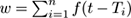
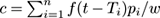
For a microcluster with center c and representing points p 1 ,p 2 ,… ,p n , with timestamps T 1 ,T 2 ,… ,T n , Den-Stream maintains the following information at time t :
-
Weight:
-
Center:
-
Radius:
 (in fact, the sums of the squares of
p
i
are kept, from which
r
can be computed when needed)
(in fact, the sums of the squares of
p
i
are kept, from which
r
can be computed when needed)
There are two types of microcluster: depending on whether the weight is larger or smaller than μ , the microcluster is called a potential core microcluster (p-microcluster) or an outlier microcluster (o-microcluster). So an outlier microcluster is a microcluster that does not (yet) have enough weight to be considered a core.
The D EN -S TREAM method has two phases, an online phase and an offine phase. Their pseudocode is shown in figure 9.2 . In the online phase, every time a new point arrives, D EN -S TREAM first tries to merge it into one of the potential microclusters. If this is not possible, it then tries to merge the point with an outlier microcluster. If the weight of the outlier microcluster has increased enough to be a potential microcluster, the microcluster is promoted. Otherwise, D EN -S TREAM starts a new outlier microcluster. The offine phase consists of removing the microclusters that have not reached a sufficient weight, and performing a batch DBSCAN clustering.
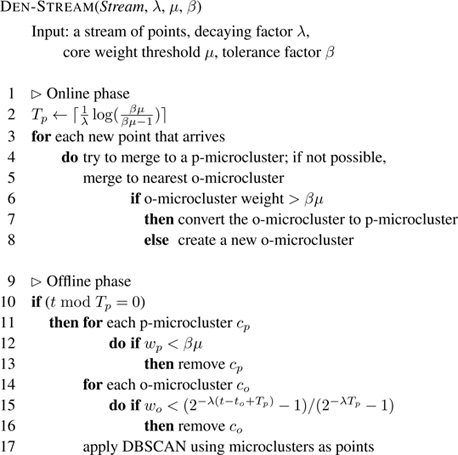
Figure 9.2
The D
EN
-S
TREAM
algorithm.
9.5 C LUS T REE
The streaming clustering algorithms presented up to now require an application of an offine phase in order to produce a cluster when requested. In contrast, C LUS T REE (Kranen et al. [ 150 ]) is an anytime clustering method, that is, it can deliver a clustering at any point in time. It is a parameter-free algorithm that automatically adapts to the speed of the stream and is capable of detecting concept drift, novelty, and outliers in the stream.
C LUS T REE uses a compact and self-adaptive index structure for maintaining stream summaries with a logarithmic insertion time. The structure is a balanced tree where each node contains a CF of a number of points, as in C LU S TREAM . This tree contains a hierarchy of microclusters at different levels of granularity. The balanced condition guarantees logarithmic access time for all microclusters.
When a new point arrives, the C LUS T REE method descends the tree to find the microcluster that is most similar to the new point. If the microcluster at the leaf reached is similar enough, then the statistics of the microcluster are updated, otherwise a new microcluster is created. But, unlike other algorithms, this process is interruptible: if new points are arriving before the leaf is reached, the point being processed is stored temporarily in an aggregate in the current inner node, and insertion is interrupted. When a new point passes later through that node, the buffered local aggregate is taken along as a “hitchhiker” and pushed further down the tree. This way, C LUS T REE can prevent the loss of points at burst times in variable-speed streams.
9.6 StreamKM++: Coresets
Given a problem and a set of input instances P , a coreset is a small weighted subset that can be used to approximate the solution to the problem. In other words, solving the problem for the coreset provides an approximate solution for the problem on P . In clustering, we can define a ( k, 𝜖 )-coreset as a pair ( S, w ) where S is a subset of P and function w assigns a nonnegative real value, the weight, to each point, in a way that the following is satisfied for each size- k subset C of P :

where cost w denotes the cost function where each point s of S is weighted by w ( s ). That is, any possible clustering chosen on P is almost equally good in S weighted by w , and vice versa. So indeed, solving the clustering problem on S and on P is approximately the same.
StreamKM++, due to Ackermann et al. [
3
], is based on this coreset idea. It uses the randomized
k
-means++ algorithm, explained in section 9.2, to create an initial set of seeds
S
= {
s
1
,…
,s
m
}. It then defines
w
(
s
i
) to be the number of points in
P
that are closer to
s
i
than to any other seed in
S
. One of the main results in [
3
] is that (
S, w
) defined in this way is a (
k
,
𝜖
)-coreset with probability 1 −
δ
, if
m
is, roughly speaking, of the form
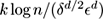 . Here,
d
is the dimension of the points in
P
and
n
is the cardinality of
P
. The dependence on
n
is very good; not so the dependence on
d
, although experimental results seem to indicate that this bound is far from tight concerning
d
.
. Here,
d
is the dimension of the points in
P
and
n
is the cardinality of
P
. The dependence on
n
is very good; not so the dependence on
d
, although experimental results seem to indicate that this bound is far from tight concerning
d
.
Furthermore, StreamKM++ places the points in a coreset tree , a binary tree that is designed to speed up the sampling according to d . The tree describes a hierarchical structure for the clusters, in the sense that the root represents the whole set of points P and the children of each node p in the tree represent a partition of the examples in p .
StreamKM++ performs an online and an offine phase. The online phase maintains a coreset of size
m
using coreset tree buckets. For a stream of
n
points, the method maintains
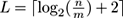 buckets
B
0
, B
1
, . . . ,
B
L
−1
. Bucket
B
0
can store less than
m
numbers, and the rest of the buckets are empty or maintain
m
points. Each bucket maintains a coreset of size
m
that represents 2
i
−1
m
points. Each time a point arrives, it is inserted in the first bucket. If this first bucket is full, then a new bucket is computed, merging
B
0
and
B
1
into a new coreset tree bucket, and moved into
B
2
. If
B
2
is not empty, this merge-and-move process is repeated until an empty bucket is reached.
buckets
B
0
, B
1
, . . . ,
B
L
−1
. Bucket
B
0
can store less than
m
numbers, and the rest of the buckets are empty or maintain
m
points. Each bucket maintains a coreset of size
m
that represents 2
i
−1
m
points. Each time a point arrives, it is inserted in the first bucket. If this first bucket is full, then a new bucket is computed, merging
B
0
and
B
1
into a new coreset tree bucket, and moved into
B
2
. If
B
2
is not empty, this merge-and-move process is repeated until an empty bucket is reached.
At any point of time the offine phase consists of applying k -means++ to a coreset of size m . The coreset of size m is obtained from the union of the buckets B 0 ,B 1 ,… ,B L −1 .
Note that StreamKM++ does not handle evolving data streams, as it has no forgetting or time-decaying mechanism.
9.7 Additional Material
Clustering is possibly the most studied task in stream mining after classification, so many other methods have been proposed besides the ones described here, including some that can be considered state-of-the-art as well. Recent comprehensive surveys are [ 84 , 185 ] and [7, chapter 10]. See also chapter 2 of [ 4 ] for an earlier survey perspective.
Streaming clustering methods were classified in [ 84 ] in five categories: partitioning methods, hierarchical methods, density-based methods, grid-based methods, and model-based methods. Among partitioning methods, DGClust and ODAC are among those with best performance. Among the hierarchical ones, improving on C LU S TREAM , are HPstream, SWClustream (which unlike C LU S TREAM can split microclusters), EStream (which explicitly models cluster dynamics by appearance, disappearance, merging, and splitting operations), and REPSTREAM (inspired by CHAMELEON). The STREAMLEADER method by Andrés-Merino and Belanche [ 15 ] was implemented on MOA and performed very competitively versus C LU S TREAM , Den-Stream, and ClusTree, both in metrics and in scalability. Among the grid-based, besides D-Stream, we can mention MR-Stream and CellTree. We refer to the surveys above for references and more details.
Given the emphasis we placed on Hoeffding Trees in the classification chapter, we mention very fast k-means (VFKM), by Domingos and Hulten [ 89 ]. It continues the philosophy of the Hoeffding Tree in that, rather than performing several passes over the same data, fresh stream data is used to simulate the further passes, and that Hoeffding’s bound is used to determine when the algorithm has seen enough data to make statistically sound choices. Like the Hoeffding Tree, VFKM has a formal guarantee that it converges to the same clustering as k -means if both work on infinite data.
9.8 Lab Session with MOA
In this lab session you will use MOA through the graphical interface to compare two clustering algorithms and evaluate them in different ways.
Exercise 9.1 Switch to the Clustering tab to set up a clustering experiment. In this tab, we have two sub-tabs, one for setup and one for visualization. This is shown in figure 9.3 . The Setup tab is selected by default. In this tab, we can specify the data stream, and the two clustering algorithms that we want to compare.
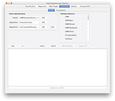
Figure 9.3
The MOA
Clustering
GUI tab.
By default, the
RandomRBFGeneratorEvents
will be used. It generates data points with class labels and weights that reflect the age of a point, depending on the chosen horizon. Since clusters move, a larger horizon yields more tail-like clusters; a small horizon yields more sphere-like clusters. Technically, the data points are obtained by generating clusters, which have a center and a maximal radius and which move through a unit cube in a random direction. At the cube boundaries, the clusters bounce off. At specific intervals, all cluster centers are shifted by 0.01 in their respective direction and points are drawn equally from each generating cluster. All clusters have the same expected number of points. This stream generator has the following parameters: the number of clusters moving through the data space, the number of generated points, the shift interval, the cluster radius, the dimensionality, and the noise rate.
The clustering algorithms that can be selected are mainly the ones we have discussed in this chapter. On the right side of the tab we can find the evaluation measures that are going to be used in the experiments.
Start by selecting clustering methods
denstream.WithDBSCAN
and
clustream.WithKmeans
. Now we are going to run and visualize our experiments. Switch to the
Visualization
tab.
Click Start to launch the experiment. The GUI will look like in figure 9.4 . The upper part of this tab offers options to pause and resume the stream, adjust the visualization speed, and choose the dimensions for x and y as well as the components to be displayed (points, micro and macro clustering, and ground truth). The lower part of the GUI displays the measured values for both settings as numbers (left side, including mean values) and the currently selected measure as a plot over the examples seen. Textual output appears in the bottom panel of the Setup tab.
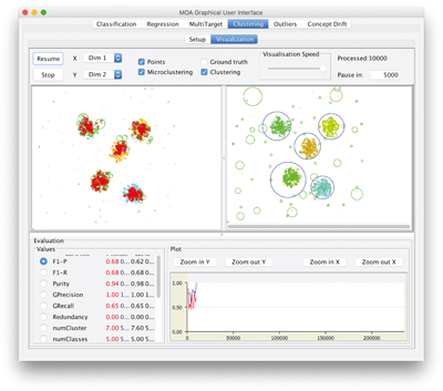
Figure 9.4
Evolving clusters in the GUI
Clustering
tab.
Click Resume to continue running the experiment.
a. What is the purity for both algorithms after 5,000 instances?
b. What is the purity for both algorithms after 10,000 instances?
Exercise 9.2 In MOA, we can easily change the parameters of the data stream generator and clustering methods.
a. Add more noise to the data, changing the noise level from 0.1 to 0.3. Which method is performing better in terms of purity after 50,000 instances?
b. Change the epsilon parameter in the Den-Stream algorithm to 0.01. Does this improve the purity results of the algorithm? Why?
Exercise 9.3 Let us compare C LU S TREAM and C LUS T REE using the default parameters. Change the methods to use in the Setup tab.
a. Which method performs better in terms of purity?
b. And in terms of CMM?
Exercise 9.4 Let us compare the performance of C LU S TREAM and C LUS T REE in the presence of noise.
a. What is the CMM of each method when there is no noise on the data stream?
b. What happens when the noise in the data stream is 5%, 10%, 15%, and 20%?