5
Dealing with Change
A central feature of the data stream model is that streams evolve over time, and algorithms must react to the change. For example, let us consider email spam classifiers, which decide whether new incoming emails are or are not spam. As classifiers learn to improve their accuracy, spammers are going to modify their strategies to build spam messages, trying to fool the classifiers into believing they are not spam. Customer behavior prediction is another example: customers, actual or potential, change their preferences as prices rise or fall, as new products appear and others fall out of fashion, or simply as the time of the year changes. The predictors in these and other situations need to be adapted, revised, or replaced as time passes if they are to maintain reasonable accuracy.
In this chapter we will first discuss the notion of change as usually understood in data streaming research, remarking on the differences with other areas that also consider changing data, then discuss possible types of change, some measures of performance used in the presence of change, and the general strategies for designing change-aware algorithms on streams (section 5.1). We will then consider methods for accurately estimating statistics of evolving data streams (section 5.2), and methods for detecting and quantifying change (section 5.3). We will conclude with some references on time-aware sketches and change detection in multidimensional streams (section 5.4).
There is a vast literature on change detection in data, and we have prioritized methods that are most applicable to data streams, easy to implement, and computationally light, and in particular those that are available in MOA. A comprehensive discussion for all types of data is [ 27 ], and an up-to-date discussion for streams is [ 116 ]. A framework for experimenting with change detection and management in MOA is presented in [ 41 ].
5.1 Notion of Change in Streams
Let us first discuss the notion of change in streams with respect to notions in other paradigms, as well as some nuances that appear when carefully defining change over time.
First, nonstationary distributions of data may also appear in batch data analysis. Data in batch datasets may also be timestamped and vary statistically over time. Algorithms may take this possibility into account when drawing conclusions from the data, but otherwise can perform several passes and examine data from before and after any given recorded time. In streaming, we cannot explicitly store all past data to detect or quantify change, and certainly we cannot use data from the future to make decisions in the present.
Second, there is some similarity to the vast field of time series analysis, where data also consists of a sequence (or a set of sequences) of timestamped items. In time series analysis, however, the analysis process is often assumed to be offine, with batch data, and without the requirements for low memory and low processing time per item inherent to streams. (Of course, we can also consider streaming, real-time time series analysis.) More importantly, in time series analysis the emphasis is often on forecasting the future evolution of the data. For example, if the average increase in sales has been 1% per month in the last six months, it is reasonable to predict that sales next month are going to be 1% higher than this month. In contrast, most of the work in streaming does not necessarily assume that change occurs in predictable ways, or has trends. Change may be arbitrary. The task is to build models describing how the world behaves right now, given what we are observing right now.
Third, the notion of change used in data streaming is different from (or a particular case of) the more general notion of “dataset shift” described in [ 182 ]. Dataset shift occurs whenever training and testing datasets come from different distributions. Streaming is one instance of this setting; for example, the predictive model we have built so far is going to be used to predict data that will arrive later, which may follow a different distribution. But it also applies to other situations, for instance where a classifier trained with batch data from a geographical region is applied to predict data coming from another region.
What do we mean exactly when we say that a data stream changes or evolves? It cannot mean that the items we observe today are not exactly the same as those that we observed yesterday. A more reasonable notion is that statistical properties of the data change more than what can be attributed to chance fluctuations. To make this idea precise, it helps to assume that the data is in fact the result of a random process that at each time generates an item according to a probability distribution that is used at that exact time, and that may or may not be the same that is used at any other given time. There is no change when this underlying generating distribution remains stationary. Change occurs whenever it varies from one time step to the next.
Recall that in the previous chapter we assumed an adversarial model, in which no randomness was assumed in the stream—only perhaps in the algorithm if it used random bits and numbers. The algorithm had to perform well even in an adversarially chosen, worst-case input. In contrast, in the randomly generated stream model, it makes sense to consider the “average case” performance of an algorithm by averaging over all possible streams according to their probability under the generating distribution. This notion of a stochastic data stream is used almost everywhere in the following chapters. For example, if the stream consists of independently generated bits with 1 having probability 1/2, then we expect to have 0s and 1s interleaved at random. The unique n -bit sequence containing n/ 2 1s first and then n/ 2 0s has negligible probability, but could determine the performance of an algorithm in the adversarial model if it turns out to be its hardest case.
Often, an additional independence assumption is implicitly or explicitly used: that the item generated at time t is independent of those generated at previous time steps. In other words, it is common to assume that the process is Markovian. This is admittedly dubious, or patently false: in many situations the stream has memory, and experiences bursts of highly correlated events. For example, a fault in a component of a system is likely to generate a burst of faults in related components. A more relaxed version of the hypothesis is that correlations are somehow short-term and that over long enough substreams the statistics are those of a Markovian process. Designing algorithms that take such autocorrelations into account is an active area of research.
Although changes in the item distribution may be arbitrary, it helps to name a few generic types, which are not exclusive within a stream. The naming is unfortunately not consistent throughout the literature. In fact, change in general is often called concept drift in the literature; we try to be more precise in the following.
- Sudden change occurs when the distribution has remained unchanged for a long time, then changes in a few steps to a significantly different one. It is often called shift .
- Gradual or incremental change occurs when, for a long time, the distribution experiences at each time step a tiny, barely noticeable change, but these accumulated changes become significant over time.
- Change may be global or partial depending on whether it affects all of the item space or just a part of it. In ML terminology, partial change might affect only instances of certain forms, or only some of the instance attributes.
- Recurrent concepts occur when distributions that have appeared in the past tend to reappear later. An example is seasonality, where summer distributions are similar among themselves and different from winter distributions. A different example is the distortions in city traffic and public transportation due to mass events or accidents, which happen at irregular, unpredictable times.
- In prediction scenarios, we are expected to predict some outcome feature Y of an item given the values of input features X observed in the item. Real change occurs when Pr[ Y | X ] changes, with or without changes in Pr[ X ]. Virtual change occurs when Pr[ X ] changes but Pr[ Y | X ] remains unchanged. In other words, in real change the rule used to label instances changes, while in virtual change the input distribution changes.
We should also distinguish the notions of outliers and noise from that of distribution change. Distinguishing true change from transient outliers and from persistent noise is one of the challenges in data stream mining and learning.
All in all, we need to consider the following requirements on data stream algorithms that build models (e.g., predictors, clusterers, or pattern miners) [ 116 ]:
- Detect change in the stream (and adapt the models, if needed) as soon as possible.
- At the same time, be robust to noise and outliers.
- Operate in less than instance arrival time and sublinear memory (ideally, some fixed, preset amount of memory).
Change management strategies can be roughly grouped into three families, or a combination thereof. They can use adaptive estimators for relevant statistics, and then an algorithm that maintains a model in synchrony with these statistics. Or they can create models that are adapted or rebuilt when a change detector indicates that change has occurred. Or they can be ensemble methods, which keep dynamic populations of models. We describe all three approaches in detail next.
The first strategy relies on the fact that many model builders work by monitoring a set of statistics from the stream and then combining them into a model. These statistics may be counts, absolute or conditional probabilities, correlations between attributes, or frequencies of certain patterns, among others. Examples of such algorithms are Naive Bayes, which keeps counts of co-occurrences of attribute values and class values, and the perceptron algorithm, which updates weights taking into account agreement between attributes and the outcome to be predicted. This strategy works by having a dynamic estimator for each relevant statistic in a way that reflects its current value, and letting the model builder feed on those estimators. The architecture is presented in Figure 5.1 .
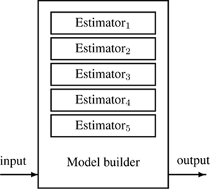
Figure 5.1
Managing change with adaptive estimators. Figure based on [
30
].
In the second strategy, one or more change detection algorithms run in parallel with the main model-building algorithm. When significant change in the stream is detected, they activate a revision algorithm, which may be different if the change is abrupt (where a new model may be built from scratch on new data) or gradual (where recalibration of the current model may be more convenient), local (affecting only parts of the model) or global (affecting all of it). A particular case is when the change is detected by observing the performance of the model—such as decreasing accuracy of a predictor. The architecture of this approach is presented in figure 5.2 .
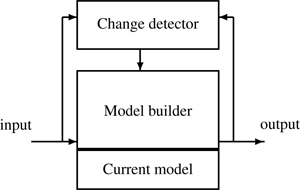
Figure 5.2
Managing change with explicit change detectors for model revision. Figure based on [
30
]
The third strategy is based on the idea of an ensemble , used to build complex classifiers out of simpler ones, covered in chapter 7. A single or several model-building algorithms are called at different times, perhaps on different subsets of the data stream. An ensemble manager algorithm contains rules for creating, erasing, and revising the models in its ensemble, as well as for combining the predictions of the models into a single prediction. Here, it is mainly the responsibility of the ensemble manager to detect and react to change, although the individual models may have this capability as well. The architecture of this approach is presented in figure 5.3 .
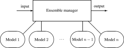
Figure 5.3
Managing change with model ensembles.
The next two sections describe some of the methods required to implement the strategies above: estimating statistics on varying streams, and detecting changes.
5.2 Estimators
An estimator algorithm estimates one or several statistics on the input data, which may change over time. We concentrate on the case in which such a statistic is (or may be rewritten as) an expected value of the current distribution of the data, which therefore could be approximated by the average of a sample of such a distribution. Part of the problem is that, with the possibility of drift, it is difficult to be sure which past elements of the stream are still reliable as samples of the current distribution, and which are outdated.
There are two kinds of estimators: those that explicitly store a sample of the data stream (we will call this store “the Memory”) and memoryless estimators. Among the former we explain the linear estimator over sliding windows. Among the latter, we explain the EWMA and the Kalman filter; other run-time efficient estimators are the autoregressive model and the autoregressive-moving-average estimator.
5.2.1 Sliding Windows and Linear Estimators
The simplest estimator algorithm for the expected value is the linear estimator , which simply returns the average of the data items contained in the Memory. An easy implementation of the Memory is a sliding window that stores the most recent W items received. Most of the time, W is a fixed parameter of the estimator; more sophisticated approaches may change W over time, perhaps in reaction to the nature of the data itself.
The memory used by estimators that use sliding windows can be reduced, for example, by using the Exponential Histogram sketch discussed in section 4.7, at the cost of some approximation error in the estimation.
5.2.2 Exponentially Weighted Moving Average
The exponentially weighted moving average (EWMA) estimator updates the estimation of a variable by combining the most recent measurement of a variable with the EWMA of all previous measurements:

where A t is the moving average at time t , x t is the latest measurement, and α ∈ (0, 1) is a parameter that reflects the weight given to the latest measurement. It is often called a decay or fading factor. Indeed, by expanding the recurrence above, we can see that the estimation at time t is

so the weight of each measurement decays exponentially fast with basis 1 − α . Larger values of α imply faster forgetting of old measurements, and smaller ones give higher importance to history.
5.2.3 Unidimensional Kalman Filter
The unidimensional Kalman filter addresses the problem of estimating the hidden state x ∈ℜ of a discrete-time controlled process that is governed by the linear stochastic difference equation

where x is observed indirectly via a measurement z ∈ℜ that is

Here w t and v t are random variables representing the process and measurement noise, respectively. They are assumed to be independent of each other and with normal probability distributions

In our setting, x t is the expected value at time t of some property of the stream items, z t is the value of the property on the item actually observed at time t , and w t , v t are the random change in x t and the observation noise in z t . The estimation y t of the state at time t is updated in the Kalman filter as follows, where P and K are auxiliary quantities:

The effectiveness of the Kalman filter in any particular application depends on the validity of the stochastic equations, of the Gaussian assumptions on the noise, and on the accuracy of the estimate of the variances Q and R .
This is a very simple version of the Kalman filter. More generally, it can be multidimensional, where x is a vector and each component of x is a linear combination of all its components at the previous time, plus noise. It also allows for control variables that we can change to influence the state and therefore create feedback loops; this is in fact the original and main purpose of the Kalman filter. And it can be extended to nonlinear measurement-to-process relations. A full exposition of the Kalman filter is [ 245 ].
5.3 Change Detection
Change detection in data is a vast subject with a long tradition in statistics; see [ 27 ]. Not all methods are apt for streaming, typically because they require several passes over the data. We cover only a few streaming-friendly ones.
5.3.1 Evaluating Change Detection
The following criteria are relevant for evaluating change detection methods. They address the fundamental trade-off that such algorithms must face [ 130 ], that between detecting true changes and avoiding false alarms. Many depend on the minimum magnitude θ of the changes we want to detect.
- Mean time between false alarms, MTFA: Measures how often we get false alarms when there is no change. The false alarm rate (FAR) is defined as 1/MTFA.
- Mean time to detection, MTD(θ ): Measures the capacity of the learning system to detect and react to change when it occurs.
- Missed detection rate, MDR(θ ): Measures the probability of not generating an alarm when there has been change.
- Average run length, ARL(θ ): This measure, which generalizes MTFA and MTD, indicates how long we have to wait before detecting a change after it occurs. We have MTFA = ARL(0) and, for θ > 0, MTD( θ ) = ARL( θ ).
5.3.2 The CUSUM and Page-Hinkley Tests
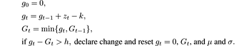
The cumulative sum (CUSUM) test [ 191 ] is designed to give an alarm when the mean of the input data significantly deviates from its previous value.
In its simplest form, the CUSUM test is as follows: given a sequence of observations { x t } t , define z t = ( x t − μ ) /σ , where μ is the expected value of the x t and σ is their standard deviation in “normal” conditions; if μ and σ are not known a priori, they are estimated from the sequence itself. Then CUSUM computes the indices and alarm:

CUSUM is memoryless and uses constant processing time per item. How its behavior depends on the parameters k and h is difficult to analyze exactly [ 27 ]. A guideline is to set k to half the value of the changes to be detected (measured in standard deviations) and h to ln(1 /δ ) where δ is the acceptable false alarm rate; values in the range 3 to 5 are typical. In general, the input z t to CUSUM can be any filter residual, for instance, the prediction error of a Kalman filter.
A variant of the CUSUM test is the Page-Hinkley test:
These formulations are one-sided in the sense that they only raise alarms when the mean increases. Two-sided versions can be easily derived by symmetry, see exercise 5.3.
5.3.3 Statistical Tests
A statistical test is a procedure for deciding whether a hypothesis about a quantitative feature of a population is true or false. We test a hypothesis of this sort by drawing a random sample from the population in question and calculating an appropriate statistic on its items. If, in doing so, we obtain a value of the statistic that would occur rarely when the hypothesis is true, we would have reason to reject the hypothesis.
To detect change, we need to compare two sources of data and decide whether the hypothesis
H
0
, that they come from the same distribution, is true. Let us suppose we have estimates
 , and
, and
 of the averages and standard deviations of two populations, drawn from equal-sized samples. If the distribution is the same in the two populations, these estimates should be consistent. Otherwise, a hypothesis test should reject
H
0
. There are several ways
to construct such a hypothesis test. The simplest one is to study the difference
of the averages and standard deviations of two populations, drawn from equal-sized samples. If the distribution is the same in the two populations, these estimates should be consistent. Otherwise, a hypothesis test should reject
H
0
. There are several ways
to construct such a hypothesis test. The simplest one is to study the difference
 , which for large samples satisfies

For example, suppose we want to design a change detector using a statistical test with a probability of false alarm of 5%, that is,

A table of the Gaussian distribution shows that P ( X < 1.96) = 0.975, so the test becomes

In the case of stream mining, the two populations are two different parts of a stream and
H
0
is the hypothesis that the two parts have the same distribution. Different implementations may differ on how they choose the parts of the stream to compare. For example, we may fix a reference window, which does not slide, and a sliding window, which slides by 1 unit at every time step. The reference window has average
 and the sliding window has average
 . When change is detected based on the two estimates, the current sliding window becomes the reference window and a new sliding window is created using the following elements. The performance of this method depends, among other parameters, on the sizes of the two windows chosen.
Instead of the normal-based test, we can perform a χ 2 -test on the variance, because

from which a standard hypothesis test can be formulated.
Still another test can be derived from Hoeffding’s bound, provided that the values of the distribution are in, say, the range [0, 1]. Suppose that we have two populations (such as windows) of sizes n 0 and n 1 . Define their harmonic mean n = 1/(1 /n 0 + 1 /n 1 ) and

We have:
- If H 0 is true and μ 0 = μ 1 , then


So the test “Is
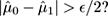 ” correctly distinguishes between identical means and means differing by at least
𝜖
with high probability. This test has the property that the guarantee is rigorously true for finite (not asymptotic)
n
0
and
n
1
; on the other hand, because Hoeffding’s bound is loose, it has small false alarm rate but large mean time to detection compared to other tests.
” correctly distinguishes between identical means and means differing by at least
𝜖
with high probability. This test has the property that the guarantee is rigorously true for finite (not asymptotic)
n
0
and
n
1
; on the other hand, because Hoeffding’s bound is loose, it has small false alarm rate but large mean time to detection compared to other tests.
5.3.4 Drift Detection Method
The drift detection method (DDM) proposed by Gama et al. [ 114 ] is applicable in the context of predictive models. The method monitors the number of errors produced by a model learned on the previous stream items. Generally, the error of the model should decrease or remain stable as more data is used, assuming that the learning method controls overfitting and that the data and label distribution is stationary. When, instead, DDM observes that the prediction error increases, it takes this as evidence that change has occurred.
More precisely, let
p
t
denote the error rate of the predictor at time
t
. Since the number of errors in a sample of
t
examples is modeled by a binomial distribution, its standard deviation at time
t
is given by
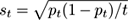 . DDM stores the smallest value
p
min
of the error rates observed up to time
t
, and the standard deviation
s
min
at that point. It then performs the following checks:
. DDM stores the smallest value
p
min
of the error rates observed up to time
t
, and the standard deviation
s
min
at that point. It then performs the following checks:
- If p t + s t ≥ p min + 2· s min , a warning is declared. From this point on, new examples are stored in anticipation of a possible declaration of change.
- If p t + s t ≥ p min + 3 · s min , change is declared. The model induced by the learning method is discarded and a new model is built using the examples stored since the warning occurred. The values for p min and s min are reset as well.
This approach is generic and simple to use, but it has the drawback that it may be too slow in responding to changes. Indeed, since p t is computed on the basis of all examples since the last change, it may take many observations after the change to make p t significantly larger than p min . Also, for slow change, the number of examples retained in memory after a warning may become large.
An evolution of this method that uses EWMA to estimate the errors is presented and thoroughly analyzed in [ 216 ].
5.3.5 ADWIN
The A DWIN algorithm (for A D aptive sliding W IN dow) [ 30 , 32 ] is a change detector and estimation algorithm based on the exponential histograms described in section 4.7. It aims at solving some of the problems in the change estimation and detection methods described before. All the problems can be attributed to the trade-off between reacting quickly to changes and having few false alarms.
Often, this trade-off is resolved by requiring the user to enter (or guess) a cutoff parameter. For example, the parameter α in EWMA indicates how to weight recent examples versus older ones; the larger the α , the more quickly the method will react to a change, but the higher the false alarm rate will be due to statistical fluctuations. Similar roles are played by the parameters in the Kalman filters and CUSUM or Page-Hinkley tests. For statistical tests based on windows, we would like to have on the one hand long windows so that the estimates on each window are more robust, but, on the other hand, short windows to detect a change as soon as it happens. The DDM method has no such parameter, but its mean time to detection depends not only on the magnitude of the change, but also on the length of the previous run without change.
Intuitively, the A DWIN algorithm resolves this trade-off by checking change at many scales simultaneously, as if for many values of α in EWMA or for many window lengths in window-based algorithms. The user does not have to guess how often change will occur or how large a deviation should trigger an alarm. The use of exponential histograms allows us to do this more efficiently in time and memory than by brute force. On the negative side, it is computationally more costly (in time and memory) than simple methods such as EWMA or CUSUM: time-per-item and memory are not constant, but logarithmic in the length of the largest window that is being monitored. So it should be used when the scale of change is unknown and this fact might be problematic.
A DWIN solves, in a well-specified way, the problem of tracking the average of a stream of bits or real-valued numbers. It keeps a variable-length window of recently seen items, with the property that the window has the maximal length statistically consistent with the hypothesis “There has been no change in the average value inside the window.” More precisely, an old fragment of the window is dropped if and only if there is enough evidence that its average value differs from that of the rest of the window. This has two consequences: one, change is reliably detected whenever the window shrinks; and two, at any time the average over the current window can be used as a reliable estimate of the current average in the stream (barring a very small or recent change that is not yet clearly visible). We now describe the algorithm in more detail.
The inputs to A DWIN are a confidence value δ ∈ (0, 1) and a (possibly infinite) sequence of real values x 1 , x 2 , x 3 , …, x t , … The value of x t is available only at time t .
The algorithm is parameterized by a test T ( W 0 , W 1 , δ ) that compares the averages of two windows W 0 and W 1 and decides whether they are likely to come from the same distribution. A good test should satisfy the following criteria:
- If W 0 and W 1 were generated from the same distribution (no change), then with probability at least 1 − δ the test says “no change.”
- If W 0 and W 1 were generated from two different distributions whose average differs by more than some quantity 𝜖 ( W 0 , W 1 , δ ), then with probability at least 1 − δ the test says “change.”
A DWIN feeds the stream of items x t to an exponential histogram. For each stream item, if there are currently b buckets in the histogram, it runs test T up to b − 1 times, as follows: For i in 1… b − 1, let W 0 be formed by the i oldest buckets, and W 1 be formed by the b − i most recent buckets, then perform the test T ( W 0 , W 1 , δ ). If some test returns “change,” it is assumed that change has occurred somewhere and the oldest bucket is dropped; the window implicitly stored in the exponential histogram has shrunk by the size of the dropped bucket. If no test returns “change,” then no bucket is dropped, so the window implicit in the exponential histogram increases by 1.
At any time, we can query the exponential histogram for an estimate of the average of the elements in the window being stored. Unlike conventional exponential histograms, the size W of the sliding window is not fixed and can grow and shrink over time. As stated before, W is in fact the size of the longest window preceding the current item on which T is unable to detect any change. The memory used by A DWIN is O (log W ) and its update time is O (log W ).
A few implementation details should be mentioned. First, it is not strictly necessary to perform the tests after each item; in practice it is all right to test every k items, of course at the risk of delaying the detection of a sudden change by time k . Second, experiments show a slight advantage in false positive rate if at most one bucket is dropped when processing any one item rather than all those before the detected change point; if necessary, more buckets will be dropped when processing further items. Third, we can fix a maximum size for the exponential histogram, so that memory does not grow unboundedly if there is no change in the stream. Finally, we need to fix a test T ; in [ 30 , 32 ] and in the MOA implementation, the Hoeffding-based test given in section 5.3.3 is used in order to have rigorous bounds on the performance of the algorithm. However, in practice, it may be better to use the other statistical tests there, which react to true changes more quickly for the same false alarm rate.
5.4 Combination with Other Sketches and Multidimensional Data
The sketches proposed in chapter 4, with the exception of exponential histograms, take into account the information in the whole data stream since the moment the sketch is initialized. This means they contain no forgetting mechanism and do not consider more recent data to be more important. It is possible and natural to combine those sketches with the estimation and change detection algorithms presented in this chapter.
For example, Papapetrou et al. [ 193 ] propose ECM, a variant of the CM-Sketch where integer counts are replaced with sliding window structures similar to Exponential Histograms. Muthukrishnan et al. [ 184 ] combine the CM-Sketch with sequential testing techniques in order to detect change in multidimensional data.
Change detection in multidimensional data streams is a challenging problem, particularly if one must scale well with the number of dimensions, and if the solution must be generic and not tailored to a specific setting. A quick solution is to reduce the problem to one dimension by monitoring the change in one or more unidimensional statistics of the data, for instance performing random projections or PCA. This typically will reduce the sensitivity to change, particularly if the change is localized in a small subspace of the data. Generic approaches for dealing with multidimensional change directly can be found in [ 82 , 153 , 201 , 237 ].
5.5 Exercises
Exercise 5.1 Discuss the differences between distribution change, outliers, anomalies, and noise.
Exercise 5.2 Propose a few strategies for managing ensembles of classifiers in the presence of distribution change. Your strategies should specify mechanisms for creating new classifiers, discarding classifiers, combining their predictions, and managing ensemble size. Think which of your strategies would be more appropriate for gradual and for sudden change. (Note: Ensemble methods will be discussed in chapter 7. Here we encourage you to give your preliminary ideas.)
Exercise 5.3 The CUSUM and Page-Hinkley tests given in the text are one-sided. Give two-sided versions that detect both increases and decreases in the average.
Exercise 5.4 a. We want to keep an array of k EWMA estimators keeping k different statistics of the stream. We know that every item in the stream contributes a 1 to at most one of the estimators, and 0 to all others. For example, the EWMAs track the frequency of k mutually exclusive types of items. The obvious strategy of updating all k estimators uses O ( k ) time per item. Describe another strategy that uses constant time per item processed and gives the same answers. Query time can be O ( k ).
b. Replace every integer entry of a CM-Sketch with an EWMA estimator with parameter α . Use the idea in the exercise above to update these estimators. What can you say about the frequency approximations that you get for every item?
c. Can you do something similar for the S PACE S AVING sketch?
Exercise 5.5 DDM has the drawback that it may take a long time to react to changes after a long period without change. Suggest a couple of ways to fix this, possibly at the cost of introducing some parameters.
Exercise 5.6 For the mathematically oriented:
- Derive the test for mean difference based on Hoeffding’s bound given in section 5.3.3.
-
Consider the implementation of A
DWIN
with the Hoeffding-based test. Analyze and describe how A
DWIN
will react to:
- A stream with abrupt change: after a long stream of bits with average μ 0 , at some time T the average suddenly changes to μ 1 ≠ μ 0 .
- Gradual shift: after a long stream of bits with average μ 0 , at time T the average starts increasing linearly so that the average at time t > T is μ t +1 = μ t + Δ, with Δ a small value.
Deduce when A DWIN will declare change, and how the window length and estimation of the average will evolve from that point on.
Exercise 5.7 For the programming oriented: program a random bit-stream generator in which the probability of getting a 1 changes abruptly or gradually after a long period with no change. Program the Page-Hinkley test, the DDM test, and the three tests in section 5.3.3 with a reference window and a sliding window. Compare the measures described in section 5.3.1 for these tests, including different window sizes for the last three tests. Do not forget to average each experiment over several random runs to get reliable estimates.