7
Ensemble Methods
Ensemble predictors are combinations of smaller models whose individual predictions are combined in some manner (say, averaging or voting) to form a final prediction. In both batch and streaming scenarios, ensembles tend to improve prediction accuracy over any of their constituents, at the cost of more time and memory resources, and they are often easy to parallelize. But in streaming, ensembles of classifiers have additional advantages over single-classifier methods: they are easy to scale; if mining a distributed stream, they do not require the several streams to be centralized toward a single site; and they can be made to adapt to change by pruning underperforming parts of the ensemble and adding new classifiers. A comprehensive and up-to-date discussion of ensembles for streams is [ 124 ].
We first discuss general methods for creating ensembles by weighting or voting existing classifiers, such as weighted majority and stacking. We then discuss bagging and boosting, two popular methods that create an ensemble by transforming the input distribution before giving it to a base algorithm that creates classifiers. Next, we discuss a few methods that use Hoeffding Trees as the base classifiers. Finally, we discuss recurrent concepts, that is, scenarios where distributions that have appeared in the past tend to reappear later, and how they can be addressed with ensembles.
7.1 Accuracy-Weighted Ensembles
A simple ensemble scheme takes N predictors C 1 , …, C N and applies some function f to combine their predictions: on every instance x to predict, the ensemble predicts f ( C 1 ( x ),… ,C N ( x )), where C i ( x ) denotes the prediction of C i for x . The predictors may be fixed from the beginning, perhaps trained offine from batch data, or trained online on the same stream.
For classification, f may simply be voting , that is, producing the most popular class among the C i ( x ). In weighted voting , each classifier C i has a weight w i attached to its vote. If we have a two-class problem, with classes in {0, 1}, weighted voting may be expressed as:

where θ is a suitable threshold. Weights may be fixed for the whole process, determined by an expert or by offine training, or vary over time. We concentrate on the latter, more interesting case.
Accuracy-Weighted Ensembles (AWE) were proposed by Wang et al. [ 244 ], and designed to mine evolving data streams using nonstreaming learners. An AWE processes a stream in chunks and builds a new classifier for each new chunk. Each time a classifier is added, the oldest one is removed, allowing the ensemble to adapt to changes. AWEs are implemented in MOA as A CCURACY W EIGHTED E NSEMBLE .
It is shown in [ 244 ] that the ensemble performs better than the base classifiers if each classifier is given weight proportional to err r − err i , where err i is the error of the i th classifier on the test set and err r is the error of a random classifier, one that predicts class c with the probability of class c in the training set. As a proxy for the test set, AWE computes these errors on the most recent chunk, assumed to be the one that is most similar to the instances that will arrive next.
Advantages of this method are its simplicity and the fact that it can be used with nonstreaming base classifiers and yet work well on both stationary and nonstationary streams. One disadvantage of the method is that the chunk size must be determined externally, by an expert on the domain, taking into account the learning curve of the base classifiers.
Variations of AWE have been presented, among others, in [ 148 , 58 ]. The one in [ 58 ] is implemented in MOA as A CCURACY U PDATED E NSEMBLE .
7.2 Weighted Majority
The Weighted Majority Algorithm, proposed by Littlestone and Warmuth [ 160 ], combines N existing predictors called “experts” (in this context), and learns to adjust their weights over time. It is similar to the perceptron algorithm, but its update rule changes the weights multiplicatively rather than additively. Unlike the perceptron, it can be shown to converge to almost the error rate of the best expert, plus a small term depending on N . It is thus useful when the number of experts is large and many of them perform poorly.
The algorithm appears in figure 7.1 . The input to the algorithm is a stream of items requiring prediction, each followed by its correct label. Upon receiving item number t , x t , the algorithm emits a prediction ŷ t for the label of x t . Then the algorithm receives the correct label y t for x t . In the algorithm the sign function returns 0 for negative numbers and 1 for nonnegative ones.
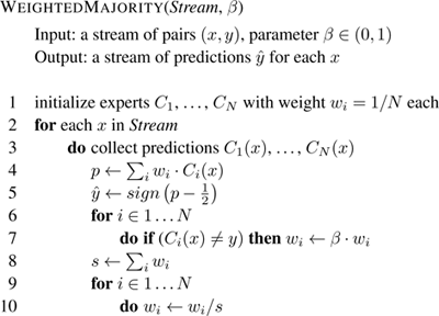
Figure 7.1
The Weighted Majority algorithm.
At time t , the algorithm predicts 1 if the sum of the experts’ predictions, weighted by the current set of weights, is at least 1/2. After that, the weight of every classifier that made a mistake is reduced by factor β . The weights are renormalized so that they add up to 1 at all times.
The intuition of the algorithm is that the weight of an expert decreases exponentially with the number of errors it makes. Therefore, if any expert has a somewhat smaller error rate than the others, its weight will decrease much more slowly, and it will soon dominate the linear combination used to make the prediction. Formalizing this argument, it was shown in [ 160 ] that no matter the order of the stream elements, at all times t ,

where err WM ,t is the number of prediction errors (examples where ŷ ≠ y ) made by Weighted Majority up to time t , and err i,t is the analogous figure for expert number i (number of examples where C i ( x ) ≠ y ). In particular, for β = 0.5, we have

In words, the number of mistakes of the Weighted Majority algorithm is only a constant factor larger than that of the best expert, plus a term that does not grow with t and depends only logarithmically on the number of experts. Observe, however, that the running time on each example is at least linear in N , unless the algorithm is parallelized.
For deterministic algorithms, the constant factor in front of min i err i,t cannot be made smaller than 2. A randomized variant is proposed in [ 160 ]: rather than predicting ŷ = sign ( p ) in line 5, predict ŷ = 1 with probability p and 0 with probability 1 − p . Randomness defeats to some extent the worst adversary choice of labels, and the constants in the bound are improved in expectation to

So, choosing β close enough to 1, the constant in front of min i err i,t can be made as close to 1 as desired. In particular, setting β = 0.5 we get

If we are interested in bounding the errors up to some time horizon
T
known in advance, we can set
 ; some calculus shows:

so the coefficient in the first term tends to 1 for large T . Weighted Majority is a special case of the Exponentiated Gradient method [ 147 ], which applies when labels and predictions are real values not in {0,1}, that is, it applies to regression problems.
7.3 Stacking
Stacking [ 247 ] is a generalization of Weighted Majority and, in fact, the most general way of combining experts. Assuming again N experts C 1 to C N , a meta-learning algorithm is used to train a meta-model on instances of the form ( C 1 ( x ),… ,C N ( x )), that is, the prediction of expert C i is considered to be feature number i . The instance x can, optionally, also be given to the meta-classifier.
The meta-learner used in stacking is often a relatively simple one such as the perceptron. Weighted Majority and Exponentiated Gradient can be seen as special cases of Stacking where a meta-learner learns a linear classifier using a multiplicative update rule instead of the additive one in the perceptron.
7.4 Bagging
The bagging method is due to Breiman [ 52 ] for the batch setting, and works in a quite different way. A base learning algorithm is used to infer M different models that are potentially different because they are trained with different bootstrap samples . Each sample is created by drawing random samples with replacement from the original training set. The resulting meta-model makes a prediction by taking the simple majority vote of the predictions of the M classifiers created in this way.
The rationale behind bagging is that voting reduces the sample variance of the base algorithm, that is, the difference among classifiers trained from different samples from the same source distribution. In fact, it works better the higher the variance among the bootstrapped classifiers.
7.4.1 Online Bagging Algorithm
In the streaming setting, it seems difficult at first to draw a sample with replacement from the stream. Yet the following property allows bootstrapping to be simulated: in a bootstrap replica, the number of copies K of each of the n examples in the training set follows a binomial distribution:

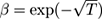
For large values of n , this binomial distribution tends to a Poisson(1) distribution, where Poisson(1) = exp(−1) /k !. Using this property, Oza and Russell proposed Online Bagging [ 189 , 190 ], which, instead of sampling with replacement, gives each arriving example a weight according to Poisson(1). Its pseudocode is given in figure 7.2 . It is implemented in MOA as O ZA B AG .
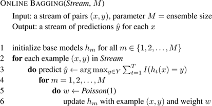
Figure 7.2
Online Bagging for
M
models. The indicator function
I
(condition) returns 1 if the condition is true, and 0 otherwise.
7.4.2 Bagging with a Change Detector
A problem with the approach above is that it is not particularly designed to react to changes in the stream, unless the base classifiers are themselves highly adaptive.
A DWIN Bagging [ 38 ], implemented in MOA as O ZA B AG ADWIN, improves on Online Bagging as follows: it uses M instances of A DWIN to monitor the error rates of the base classifiers. When any one detects a change, the worst classifier in the ensemble is removed and a new classifier is added to it. This strategy is sometimes called “replace the loser.”
7.4.3 Leveraging Bagging
An experimental observation when using online bagging is that adding more randomness to the input seems to improve performance. Since adding randomness increases the diversity or variance of the base classifiers, this agrees with the intuition that bagging benefits from higher classifier variance.
Additional randomness can be introduced by sampling with distributions other than Poisson(1). For example, Lee and Clyde [ 155 ] use the Γ(1,1) distribution to obtain a Bayesian version of bagging. Note that Γ(1,1) equals Exp (1). Bühlmann and Yu [ 60 ] propose subbagging, that is, using resampling without replacement.
Leveraging Bagging [ 36 ] samples the stream with distribution Poisson( λ ), where λ ≥ 1 is a parameter of the algorithm. Since the Poisson distribution has variance (and mean) λ , this does increase the variance in the bootstrap samples with respect to regular Online Bagging. It is implemented in MOA as L EVERAGING B AG .
Besides adding randomness to the input, Leveraging Bagging also adds randomization at the output of the ensemble using output codes. Dietterich and Bakiri [ 87 ] introduced a method based on error-correcting output codes, which handles multiclass problems using only a binary classifier. The classes assigned to each example are modified to create a new binary classification of the data induced by a mapping from the set of classes to {0,1}. A variation of this method by Schapire [ 222 ] presented a form of boosting using output codes. Leveraging Bagging uses random output codes instead of deterministic codes. In standard ensemble methods, all classifiers try to predict the same function. However, using output codes, each classifier will predict a different function. This may reduce the effects of correlations between the classifiers, and increase the diversity of the ensemble.
Leveraging Bagging also incorporates the “replace the loser” strategy in A DWIN Bagging. Experiments in [ 36 ] show that Leveraging Bagging improves over regular Online Bagging and over A DWIN Bagging.
7.5 Boosting
Like bagging, boosting algorithms combine multiple base models trained with samples of the input to achieve lower classification error. Unlike bagging, the models are created sequentially rather than in parallel, with the construction of each new model depending on the performance of the previously constructed models. The intuitive idea of boosting is to give more weight to the examples misclassified by the current ensemble of classifiers, so that the next classifier in the sequence pays more attention to these examples. AdaBoost.M1 [ 108 ] is the most popular variant of batch boosting.
This sequential nature makes boosting more difficult than bagging to transfer to streaming. For online settings, Oza and Russell [ 189 , 190 ] proposed Online Boosting , an online method that, rather than building new models sequentially each time a new instance arrives, instead updates each model with a weight computed depending on the performance of the previous classifiers. It is implemented in MOA as O ZA B OOST . Other online boosting-like methods are given in [ 53 , 54 , 65 , 85 , 197 , 243 , 259 ].
According to [ 187 ], among others, in the batch setting boosting often outperforms bagging, but it is also more sensitive to noise, so bagging gives improvements more consistently. Early studies comparing online boosting and online bagging methods, however, seemed to favor bagging [ 38 , 189 , 190 ]. An exception is [ 100 ], which reported the Arc-x4 boosting algorithm [ 53 ] performing better than online bagging. Additional studies comparing the more recent variants would be interesting. Also, it is unclear how to make a boosting algorithm deal with concept drift, because a strategy such as “replace the loser” does not seem as justifiable as in bagging.
7.6 Ensembles of Hoeffding Trees
Since Hoeffding Trees are among the most useful and best-studied streaming classifiers, several ways of combining them into ensembles have been proposed.
7.6.1 Hoeffding Option Trees
Hoeffding Option Trees (HOT) [ 198 ] represent ensembles of trees implicitly in a single tree structure. A HOT contains, besides regular nodes that test one attribute, option nodes that apply no test and simply branch into several subtrees. When an instance reaches an option node, it continues descending through all its children, eventually reaching several leaves. The output of the tree on an instance is then determined by a vote among all the leaf nodes reached.
Option nodes are introduced when the splitting criterion of the Hoeffding Tree algorithm seems to value several attributes similarly after receiving a reasonable number of examples. Rather than waiting arbitrarily long to break a tie, all tied attributes are added as options. In this way, the effects of limited lookahead and instability are mitigated, leading to a more accurate model.
We omit several additional details given in [ 198 ] and implemented in the MOA version of HOT, named H OEFFDING O PTION T REE . The voting among the leaves is weighted rather than using simple majority voting. Strategies to limit tree growth are required, as option trees have a tendency to grow very rapidly if not controlled. HOTs for regression, with subtle differences in the construction process, were proposed in [ 140 ].
7.6.2 Random Forests
Breiman [ 55 ] proposed Random Forests in the batch setting as ensembles of trees that use randomization on the input and on the internal construction of the decision trees. The input is randomized by taking bootstrap samples, as in standard bagging. The construction of the trees is randomized by requiring that at each node only a randomly chosen subset of the attributes can be used for splitting. The subset is usually quite small, with a size such as the square root of the total number of attributes. Furthermore, the trees are grown without pruning. Random Forests are usually among the top-performing classifier methods in many batch tasks.
Streaming implementations of random forests have been proposed by, among others, Abdulsalam et al. [ 2 ], who did not exactly use Hoeffding Trees but another type of online tree builder. An implementation using Hoeffding Trees that exploits GPU computing power is given in [ 167 ]. These and most other implementations of streaming Random Forests use the “replace the loser” strategy for dealing with concept drift.
Unfortunately, none of these Random Forest algorithms have been able to compete effectively with the various bagging- and boosting-based algorithms mentioned before. Recently, however, Gomes et al. [ 125 ] presented the Adaptive Random Forest (ARF) algorithm that appears as a strong contender. In contrast to previous attempts at replicating Random Forests for data stream learning [ 124 ], ARF includes an effective resampling method and adaptive operators that can cope with different types of concept drift without complex optimizations for different datasets. The parallel implementation of ARF presented in [ 125 ] shows no degradation in terms of classification performance compared to a serial implementation, since trees and adaptive operators are independent of one another.
7.6.3 Perceptron Stacking of Restricted Hoeffding Trees
An observation made repeatedly in ML is that, often, complicated models are outperformed by simpler models that do not attempt to model complex interactions among attributes. This possibility was investigated for ensembles of Hoeffding Trees by Bifet et al. [ 31 ]. In contrast with Random Forests of full Hoeffding Trees, they proposed to use stacking with the perceptron algorithm using small trees.
More precisely, their algorithm enumerates all the subsets of attributes of size k and learns a Hoeffding Tree on each. These trees are the input to a stacking algorithm that uses the perceptron algorithm as a meta-learner. Growing the trees is fast, as each tree is small, and we expect the meta-learner to end up assigning large weights to the best combination(s) of k attributes.
Since there are
 sets of size
k
among
n
attributes, only small values of
k
are feasible for most values of
n
. For
k
= 1 the algorithm becomes the perceptron, but
k
= 2 is found to be practical for medium-size datasets. To
deal with concept drift, the method adds an A
DWIN
change detector to each tree. When the error rate of a tree changes significantly, the tree is reset and a new tree with that attribute combination is learned. The method is shown in [
31
] to perform better than A
DWIN
Bagging on simple synthetic datasets, which suggests that it could perform well in cases where the key to prediction is not a complex combination of attributes.
sets of size
k
among
n
attributes, only small values of
k
are feasible for most values of
n
. For
k
= 1 the algorithm becomes the perceptron, but
k
= 2 is found to be practical for medium-size datasets. To
deal with concept drift, the method adds an A
DWIN
change detector to each tree. When the error rate of a tree changes significantly, the tree is reset and a new tree with that attribute combination is learned. The method is shown in [
31
] to perform better than A
DWIN
Bagging on simple synthetic datasets, which suggests that it could perform well in cases where the key to prediction is not a complex combination of attributes.
This method is implemented in MOA as L IM A TT C LASSIFIER .
7.6.4 Adaptive-Size Hoeffding Trees
The Adaptive-Size Hoeffding Tree (ASHT) method [ 38 ], implemented in MOA as O ZA B AG ASHT, creates an ensemble of Hoeffding trees with the following restrictions:
- Each tree in the ensemble has an associated value representing the maximum number of internal nodes it can reach.
- After a node split occurs in a tree, if its size exceeds its associated value, then the tree is reset to a leaf.
If there are N trees in the ensemble, one way to assign the maximum sizes is to choose powers of, say, 2: 2, 4, … up to 2 k . The intuition behind this method is that smaller trees adapt more quickly to changes, and larger trees perform better during periods with little or no change, simply because they were built using more data. Trees limited to size s will be reset about twice as often as trees limited to size 2 s . This creates a set of different reset speeds for an ensemble of such trees, and therefore a subset of trees that are a good approximation for the current rate of change.
The output of the ensemble can be the majority vote among all trees, although [ 38 ] finds experimentally that it is better to weight them in inverse proportion to the square of their errors. The error of each tree is monitored by an EWMA estimator.
It is important to note that resets will happen all the time, even for stationary datasets, but this behavior should not harm the ensemble’s predictive performance.
7.7 Recurrent Concepts
In many settings, the stream distribution evolves in such a way that distributions occurring in the past reappear in the future. Streams with clear daily, weekly, or yearly periodicity (such as weather, customer sales, and road traffic) are examples, but reoccurrence may also occur in nonperiodic ways.
Recurring or recurrent concept frameworks have been proposed [ 112 , 127 , 143 , 219 ] for these scenarios. Proposals differ in detail, but the main idea is to keep a library of classifiers that have been useful in the past but have been removed from the ensemble, for example because at some point they underperformed. Still, their accuracy is rechecked periodically in case they seem to be performing well again, and if so, they are added back to the ensemble.
Far fewer examples are required to estimate the accuracy of a classifier than to build a new one from scratch, so this scheme trades training time for memory. Additional rules are required for discarding classifiers from the library when it grows too large.
The RCD recurrent concept framework by Gonçalves and de Barros [ 143 ] is available as a MOA extension.
7.8 Lab Session with MOA
In this lab session we will use MOA through the graphical interface with various ensemble streaming classifiers and evolving streams.
Exercise 7.1
We begin with a non-evolving scenario. The
RandomRBF
data generator creates a random set of centers for each class, each comprising a weight, a central point per attribute, and a standard deviation. It then generates instances by choosing a center at random (taking the weights into consideration), which determines the class, and randomly choosing attribute values and an offset from the center. The overall vector is scaled to a length that is randomly sampled from a Gaussian distribution around the center.
a. What is the accuracy of Naive Bayes on a
RandomRBFGenerator
stream of 1,000,000 instances with default values, using
Prequential
evaluation and the
BasicClassificationPerformanceEvaluator
?
b. What is the accuracy of the Hoeffding Tree in the same situation?
Exercise 7.2
MOA’s Hoeffding Tree algorithm can use different prediction methods at the leaves. The default is an adaptive Naive Bayes method, but a majority class classifier can be used instead by specifying
-l (trees.HoeffdingTree -l MC)
. You can set this up in MOA’s
Configure
interface (you need to scroll down).
a. What is the accuracy of the Hoeffding Tree when a majority class classifier is used at the leaves?
b. What is the accuracy of the
OzaBag
bagging classifier?
Exercise 7.3
Now let us use an evolving data stream. The rate of movement of the centroids of the
RandomRBFGeneratorDrift
generator can be controled using the
speedChange
parameter.
a. Use the Naive Bayes classifier on a
RandomRBFGeneratorDrift
stream of 1,000,000 instances with 0.001 change speed. Use again
BasicClassificationPerformanceEvaluator
for prequential evaluation. What is the accuracy that we obtain?
b. What is the accuracy of a Hoeffding Tree under the same conditions?
c. What is the corresponding accuracy of
OzaBag
?
Exercise 7.4 The Hoeffding Adaptive Tree adapts to changes in the data stream by constructing tentative “alternative branches” as preparation for changes, and switching to them if they become more accurate. A change detector with theoretical guarantees (ADWIN) is used to check whether to substitute alternative subtrees.
a. What is the accuracy of
HoeffdingAdaptiveTree
in the above situation?
b. What is the accuracy for
OzaBagAdwin
, the ADWIN adaptive bagging technique?
c. Finally, what is the accuracy for
LeveragingBag
method?
Exercise 7.5
Besides data streams, MOA can also process ARFF files. We will use the
covtypeNorm.arff
dataset, which can be downloaded from the MOA website. Run the following task, which uses the Naive Bayes classifier:
EvaluatePrequential
-s (ArffFileStream -f covtypeNorm.arff)
-e BasicClassificationPerformanceEvaluator
-i 1000000 -f 10000
You will have to copy and paste this into the
Configure
text box, because you cannot specify an
ArffFileStream
in MOA’s interactive interface. Also, the default location for files is the top level of the MOA installation folder—you will probably find the model files
modelNB.moa
and
modelHT.moa
that you made in the last session lab there—so you should either copy the ARFF file there or use its full pathname in the command.
a. What is the accuracy of Naive Bayes on this dataset?
b. What is the accuracy of a Hoeffding Tree on the same dataset?
c. Finally, what is the accuracy of Leveraging Bagging?
d. Which method is fastest on this data?
e. Which method is most accurate?