12
The Graphical User Interface
The MOA Graphical User Interface (GUI) allows using MOA via menu selection and form filling. It contains several tabs on the top, for four learning tasks: Classification, regression, clustering, and outlier detection. In this chapter we describe the main options for evaluation, classification, and clustering; readers are encouraged to explore more, and read the MOA documentation for more detail on, for example, the parameters available for each method.
12.1 Getting Started with the GUI
The GUI for configuring and running tasks is invoked with the command:
bin/moa.sh
in Linux or Mac, and
bin\moa.bat
in Windows. These commands call the GUI using
java -Xmx1G … moa.gui.GUI
There are several tabs, for classification, regression, clustering, and outlier detection. In the following sections we are going to describe how to use them.
12.2 Classification and Regression
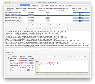
The classification and regression tabs in MOA contain four different components as seen in Figure 12.1 :
- Configure Current Task
- List of Tasks
- Output Panel
- Evaluation Measure and Chart Output Panel.

Figure 12.1
The MOA Graphical User Interface.
To use the classification GUI, first we need to configure a task, then run it, and finally see the results in the output panels.
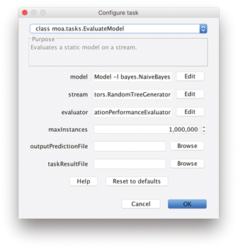
We can click Configure to set up a task, modify the parameters of the task (see Figure 12.2 ), and when ready we can launch a task clicking Run . Several tasks can be run concurrently. We can click on different tasks in the list and control them using the buttons below. If textual output of a task is available it will be displayed in the bottom half of the GUI, and can be saved to disk. If graphical output is available it will be displayed in the bottom chart display.

Figure 12.2
Options to set up a task in MOA.
Note that the command line text box displayed at the top of the window represents textual commands that can be used to run tasks on the command line as described in the next chapter. The text can be selected then copied onto the clipboard. At the bottom of the GUI there is a graphical display of the results. It is possible to compare the results of two different tasks: The current task is displayed in red, and the previously executed one is in blue.
12.2.1 Tasks
The main tasks in MOA are the following:
- WriteStreamToARFFFile Outputs a stream to an ARFF file. ARFF is a convenient data format used by the WEKA project [ 107 ] that extends the CSV format with a header specifying attribute types, names, and values.
- MeasureStreamSpeed Measures the speed of a stream.
- LearnModel Learns a predictive model from a stream.
- EvaluateModel Evaluates a static predictive model on a stream.
- EvaluatePeriodicHeldOutTest Evaluates a classifier on a stream by periodically testing on a holdout set.
- EvaluateInterleavedTestThenTrain Evaluates a classifier on a stream by testing then training with each instance in sequence. There is no forgetting mechanism so all instances are equally important in the evaluation.
- EvaluatePrequential Evaluates a classifier on a stream by testing then training with each example in sequence. It may optionally use a sliding window or a fading factor as forgetting mechanisms.
- EvaluatePrequentialCV Evaluates a classifier on a stream by doing k -fold distributed cross-validation; each time a new instance arrives, it is used for testing in one classifier selected randomly, and trained using the others. It may optionally use a sliding window or a fading factor as forgetting mechanisms.
- EvaluateInterleavedChunks Evaluates a classifier on a stream by testing then training with chunks of data in sequence.
Evaluation methods were defined in Section 6.1.
12.2.2 Data Feeds and Data Generators
MOA streams are built using generators, reading ARFF files, joining several streams, or filtering streams. They allow to simulate a potentially infinite sequence of data. The following ones are implemented:
- ArffFileStream Reads a stream from an ARFF file.
- ConceptDriftStream Creates a stream with concept drift by smoothly merging two streams that have the same attributes and classes.
MOA models concept drift in a data stream as a weighted mixture of two existing streams that describe the data distributions before and after the drift. MOA uses the sigmoid function as a simple and practical solution to define the merging of two streams to simulate drift.
We see from Figure 3.5 in Section 3.2.1 that the sigmoid function

has a derivative at the point p such that f ′( p ) = s/ 4. The tangent of angle α is equal to this derivative, tan α = s/ 4. We observe that tan α = 1 /w , and as s = 4 tan α then s = 4 /w . So the parameter s in the sigmoid gives the length of w and the angle α . In this sigmoid model we only need to specify two parameters: the point of change p , and the length of change w . Note that for any positive real number β

and that f ( p + β · w ) and f ( p − β · w ) are constant values that do not depend on p and w . We have, for example,

Given two data streams
 is defined as the data stream built joining the two data streams
a
and
b
, where
p
is the point of change,
w
is the length of change and

We observe the following properties, if a ≠ b :

In order to create a data stream with multiple concept changes, we can build new data streams joining different concept drifts:

- ConceptDriftRealStream Generator that creates a stream with concept drift by merging two streams that have different attributes and classes. The new stream contains the attributes and classes of both streams.
- FilteredStream A stream that is obtained from a stream filtered by a filter, for example AddNoiseFilter .
- AddNoiseFilter Adds random noise to examples in a stream. To be used with FilteredStream only.
- generators.AgrawalGenerator Generates one of ten different pre-defined loan functions.
This generator was introduced by Agrawal et al. in [ 8 ]. It was a common source of data for early work on scaling up decision tree learners. The generator produces a stream containing nine attributes, six numeric ones and three categorical ones. Although not explicitly stated by the authors, a sensible guess is that these attributes describe hypothetical loan applications. There are ten functions defined for generating binary class labels from the attributes. Presumably these determine whether the loan should be approved or not.
A source code in C is publicly available. The built-in functions are based on the cited paper (page 924), which turn out to be functions pred20 thru pred29 in the public C implementation. The perturbation function works as in the C implementation rather than the description in paper.
- generators.HyperplaneGenerator Generates a problem of predicting class of a rotating hyperplane.
The problem was used as testbed for CVFDT versus VFDT in [
138
]. A hyperplane in
d
-dimensional space is the set of points
x
∈ℜ
d
that satisfy
 , where
x
i
is the ith coordinate of point
x
. Point examples for which
 are labeled positive, and point examples for which
 are labeled negative. Hyperplanes are useful for simulating time-changing concepts, because we can change the orientation and position of the hyperplane in a smooth manner by changing the relative values of the weights. We add change to this dataset adding drift to each weight attribute,
w
i
=
w
i
+
dσ
, where
σ
is the probability that the direction of change is reversed and
d
is the speed of change.
- generators.LEDGenerator Generates a problem of predicting the digit displayed on a 7-segment LED display.
This data source originates from the CART book [ 56 ]. The goal is to predict the digit displayed on a seven-segment LED display, where each attribute has a 10% chance of being inverted. It has an optimal Bayes classification rate (rate of the best possible classifier) of 74%. The particular configuration of the generator used for experiments (led) produces 24 binary attributes, 17 of which are irrelevant.
- generators.LEDGeneratorDrift Generates a problem of predicting the digit displayed on a 7-segment LED display with drift.
- generators.RandomRBFGenerator Generates a random radial basis function stream.
This generator was devised to offer an alternate complex concept type that is not straightforward to approximate with decision trees. The RBF (Radial Basis Function) generator works as follows: A fixed number of random clusters are generated. Each cluster has a random center, a standard deviation, a class label and a weight. New examples are generated by selecting a cluster with probability proportional to its weight, then generating a point from a Gaussian distribution with the center at the cluster’s center and the cluster’s standard deviation along every axis. This effectively creates a normally distributed hypersphere of examples surrounding each center, with varying densities. Only numeric attributes are generated. The chosen cluster also determines the class label of the example.
- generators.RandomRBFGeneratorDrift Generates a random radial basis function stream with drift. Drift is introduced by moving the centers at constant speed.
- generators.RandomTreeGenerator Generates a stream based on a randomly generated tree.
This generator is based on that proposed in [ 88 ] and produces concepts that should favor decision tree learners. It builds a decision tree by choosing attributes to split at random and assigning a random class label to each leaf. Once the tree is built, examples in the stream are generated by assigning uniformly distributed random values to attributes, which then determine the class label via the tree. The generator has parameters to control the number of classes, attributes, nominal attribute labels, and the depth of the tree.
Noise can be introduced in the examples after generation. In the case of discrete attributes and the class label, a probability of noise parameter determines the chance that any particular value is switched to something other than the original value. For numeric attributes, a degree of random noise is added to all values, drawn from a random Gaussian distribution with standard deviation equal to the standard deviation of the original values multiplied by noise probability.
- generators.SEAGenerator Generates SEA concepts functions.
This generator was proposed in [ 233 ] to study reaction to abrupt concept drift. The stream is generated using three attributes, and only the first two are relevant. All three attributes have values between 0 and 10. The points in the stream are divided into four blocks with different concepts. In each block, the 0/1 class is determined by the inequality f 1 + f 2 ≤ θ , where f 1 and f 2 represent the first two attributes and θ is a threshold value. The most usual threshold values for the four classes are 9, 8, 7 and 9.5.
- generators.STAGGERGenerator Generates STAGGER concept functions, introduced by Schlimmer and Granger in [ 223 ].
The STAGGER concepts are boolean functions of three attributes encoding objects: size (small, medium, large), shape (circle, triangle, rectangle), and color (red, blue, green). A concept is a conjunction or disjunction of two attributes, such as (color=red and size=small) or (color=green or shape=circle) .
- generators.WaveformGenerator Generates a problem of predicting one of three waveform types.
It shares its origin with the LED dataset. The goal of the task is to differentiate between three different classes of waveform, each of which is generated from a combination of two or three base waves. The optimal Bayes classification rate is known to be 86%. There are two versions of the problem, wave21 which has 21 numeric attributes, all of which include noise, and wave40, which introduces 19 additional irrelevant attributes.
- generators.WaveformGeneratorDrift Generates a problem of predicting one of three waveform types, with drift.
12.2.3 Bayesian Classifiers
- NaiveBayes Performs classic bayesian prediction making the naive assumption that all attributes are independent. It has been described in Section 6.2.3.
- NaiveBayesMultinomial The Multinomial Naive Bayes classifier is described in 6.2.4.
12.2.4 Decision Trees
-
HoeffdingTree
Decision tree inducer for data streams without change, described in Section 6.3.2. To use majority class learners at the leaves, use
HoeffdingTree -l MC. - DecisionStump Decision tree with a single inner node, so that only one attribute is tested to predict an instance.
-
HoeffdingOptionTree
Hoeffding Option Trees, described in Section 7.6.1. It is possible to choose the type of classifier placed at the leaves: Majority class, Naive Bayes, or Naive Bayes Adaptive. By default, the option selected is Naive Bayes Adaptive, since it tends to give best results; it monitors the error rate of the majority class and Naive Bayes predictors, and switches from one to the other tracking the one with better rate on recent instances. To run experiments using a majority class learner at leaves, use
HoeffdingOptionTree -l MC. - HoeffdingAdaptiveTree Decision tree inducer for evolving data streams, described in Section 6.3.5.
- AdaHoeffdingOptionTree Adaptive Hoeffding Option Tree for streaming data with Naive Bayes Adaptive classifiers at the leaves [ 38 ]. An Adaptive Hoeffding Option Tree is a Hoeffding Option Tree with the following improvement: Each leaf stores an estimation of the current error, estimated using an EWMA counter with α = 0.2. The weight of each node in the voting process is proportional to the square of the inverse of the error.
12.2.5 Meta Classifiers (Ensembles)
- OzaBag Incremental online bagging by Oza and Russell, described in Section 7.4.1.
- OzaBoost Incremental online boosting by Oza and Russell [ 190 ].
- OCBoost Online Coordinate Boosting by Pelossof et al. [ 197 ]. An online boosting algorithm for adapting the weights of a boosted classifier, which yields a closer approximation to Freund and Schapire’s AdaBoost algorithm. The weight update procedure is derived by minimizing AdaBoost’s loss when viewed in an incremental form. This boosting method may be reduced to a form similar to Oza and Russell’s algorithm.
- OzaBagASHT Bagging using Hoeffding trees, each with a maximum size value, and described in Section 7.6.4. The base learner must be ASHoeffdingTree, a Hoeffding Tree with a maximum size value.
- OzaBagADWIN Bagging using A DWIN , described in Section 7.4.2.
- AccuracyWeightedEnsemble , described in Section 7.1.
- AccuracyUpdatedEnsemble , a variant by Brzezinski and Stefanowski [ 58 ] of the method described in Section 7.1.
- LimAttClassifier , ensemble combining Restricted Hoeffding Trees using Stacking with a Perceptron, described in Section 7.6.3.
-
LeveragingBag
Leveraging Bagging for evolving data streams using ADWIN, described in Section 7.4.3. There are four different versions of this algorithm:
- Leveraging Bagging ME, using weight 1 if misclassified, otherwise error/(1-error).
- Leveraging Bagging Half, using resampling without replacement half of the instances.
- Leveraging Bagging WT, without taking out all instances.
- Leveraging Subagging, using resampling without replacement.
The “-o” option can be used to use Random Output codes.
- TemporallyAugmentedClassifier Wrapper that includes labels of previous instances into the training data. This enables a classifier to exploit potential label auto-correlation. See Section 6.2.2.
12.2.6 Function Classifiers
- MajorityClass always predicts the class that has been observed most frequently in the training data.
- NoChange It predicts the class that has been observed in the last instance used to train the model.
- Perceptron , single perceptron classifier. Performs the classic multiclass perceptron learning, incrementally.
- SGD Implements stochastic gradient descent for learning various linear models: binary class SVM, binary class logistic regression, and linear regression.
- SPegasos Implements the stochastic variant of the Pegasos (Primal Estimated sub-GrAdient SOlver for SVM) method of Shalev-Shwartz et al. [ 226 ].
12.2.7 Drift Classifiers
-
SingleClassifierDrift
classifier for handling concept drift data streams, based on using a change detector to monitor the error of the classifier. When
the change detector raises a warning signal, a new classifier is created; and when a change signal is raised, the current classifier is replaced by the new one. It is the strategy in the DDM method of Gama et al. [
114
], described in Section 5.3.4. There are several drift detection methods that can be used:
- CusumDM and PageHinkleyDM , as seen in Section 5.3.2.
- DDM , seen in Section 5.3.4.
- EDDM , based on using the estimated distribution. of the distances between classification errors, presented in [ 22 ].
- ADWINChangeDetector , as seen in Section 5.3.5.
- EWMAChartDM , based on using an exponentially weighted moving average (EWMA) chart [ 216 ], mentioned in Section 5.3.4.
- GeometricMovingAverageDM , based in the use of a geometric moving average estimation.
- HDDM_A_Test and HDDM_W_Test , based on using Hoeffding’s bounds presented in [ 44 ].
- SEEDChangeDetector , based on detecting volatility shift, presented in [ 136 ].
- SeqDrift1ChangeDetector and SeqDrift2ChangeDetector , the first one based on comparing data in a sliding window and data in a repository, and the second one based in comparing data in a reservoir and data in a repository, presented in [ 196 , 220 ].
- STEPD , based on using a statistical test of equal proportions, presented in [ 186 ].
12.2.8 Active Learning Classifiers
- ActiveClassifier Classifier for active learning that aims at learning an accurate model while not requesting more labels than allowed by its budget. This classifier can use several active learning strategies that explicitly handle concept drift, described in Section 6.8.
12.3 Clustering
The Clustering tab in MOA has the following main components:
- Data generators for stream clustering on evolving streams (including events like novelty, merge, etc.),
- a set of state-of-the-art stream clustering algorithms,
- evaluation measures for stream clustering, and
- visualization tools for analyzing results and comparing different settings.
12.3.1 Data Feeds and Data Generators
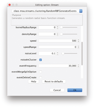
Figure 12.3 shows a screenshot of the configuration dialog for the RBF data generator with events. Generally the dimension, number, and size of clusters can be set as well as the drift speed, decay horizon (aging), and noise rate. Events constitute changes in the underlying data model such as cluster growth, cluster merging, or creation of a new cluster. Using the event frequency and the individual event weights, one can study the behavior and performance of different approaches on various settings. Finally, the settings for the data generators can be stored and loaded, which offers the opportunity of sharing settings and thereby providing benchmark streaming datasets for repeatability and comparison.

Figure 12.3
Option dialog for the RBF data generator. By storing and loading settings, streaming datasets can be shared for benchmarking, repeatability and comparison.
12.3.2 Stream Clustering Algorithms
Currently MOA contains several stream clustering methods, including:
- StreamKM++, described in Section 9.2.
- CluStream, described in Section 9.3.
- ClusTree, described in Section 9.5.
- Den-Stream, described in Section 9.5.
- CobWeb. A hierarchical clusterer, and one of the first incremental methods for clustering data, due to Fisher [ 102 ].
12.3.3 Visualization and Analysis
After the evaluation process is started, several options for analyzing the outputs are possible:
- The stream can be stopped and the current (micro)clustering result can be passed as a dataset to the WEKA explorer for further analysis or mining;
- the evaluation measures, which are evaluated at configurable time intervals, can be stored as a CSV file to obtain graphs and charts offine using a program of choice;
- finally, both the clustering results and the corresponding measures can be visualized online within MOA.
MOA allows the simultaneous configuration and evaluation of two different setups for direct comparison, for example of two different algorithms on the same stream or the same algorithm on streams with different noise levels, and so on.
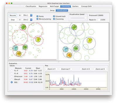
The visualization component allows to visualize the stream as well as the clustering results, choose dimensions for multidimensional data, and compare experiments with different settings in parallel. Figure 12.4 shows a screenshot of the visualization tab. In this screenshot, two different settings of the CluStream algorithm are compared on the same stream setting, including merge/ split events every 50000 examples, and four measures were chosen for online evaluation (F1, Precision, Recall, and SSQ).

Figure 12.4
Visualization tab of the MOA clustering GUI.
The upper part of the GUI offers options to pause and resume the stream, adjust the visualization speed, choose the dimensions for x and y as well as the components to be displayed (points, micro- and macro- clustering and ground truth). The lower part of the GUI displays the measured values for both settings as numbers (left side, including mean values) and the currently selected measure as a plot over the processed examples (right, SSQ measure in this example).